21 Regression Analysis

21.1 Regression

We use the following synthetic data, which has the important advantage that we know the ground truth.

The underlying function is the following

f = function(x) (1 + 10*x - 5*x^2)*sin(10*x)
curve(f, lwd = 2)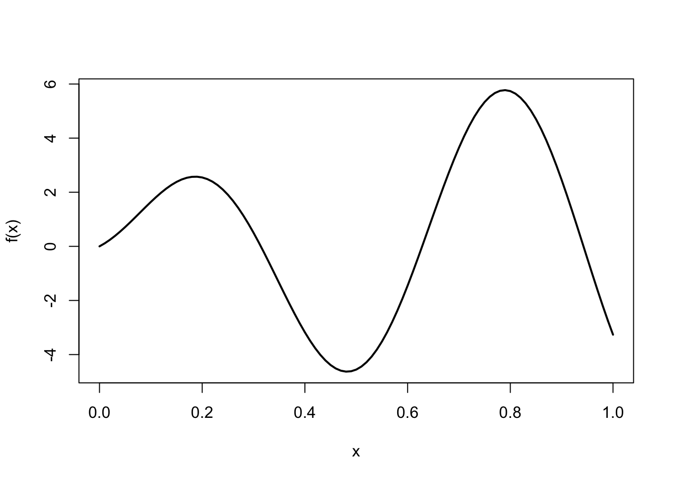

We then sample the function uniformly at random on the unit interval and then observe the corresponding values albeit with additive Gaussian noise

n = 200 # sample size
x = runif(n) # the predictor variable
x = sort(x) # we sort x for ease of plotting
y = f(x) + 0.5*rnorm(n) # the response variable

We will use the following helper function to reset the plot. It displays a scatterplot of the data together with the underlying function in dashed line.

plot_reset = function(){
  plot(x, y, pch = 16, cex = 0.7)
  curve(f, lty = 2, add = TRUE)
}
plot_reset()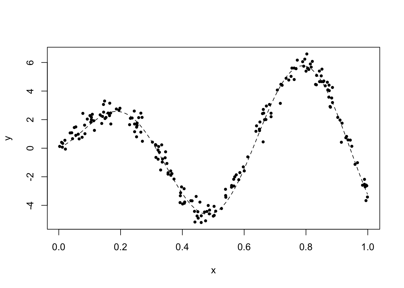

21.1.1 Kernel smoothing

We use the Gaussian kernel and try a few different values for the bandwidth. Notice how the last two estimators are grossly biased near \(x = 1\).

plot_reset()
x_new = seq(0, 1, len = 1000) # for plotting purposes

h = 0.05 # bandwidth
fit = ksmooth(x, y, "normal", bandwidth = h, x.points = x_new)
lines(x_new, fit$y, col = "darkred", lwd = 2)

h = 0.15 # bandwidth
fit = ksmooth(x, y, "normal", bandwidth = h, x.points = x_new)
lines(x_new, fit$y, col = "darkgreen", lwd = 2)

h = 0.25 # bandwidth
fit = ksmooth(x, y, "normal", bandwidth = h, x.points = x_new)
lines(x_new, fit$y, col = "darkblue", lwd = 2)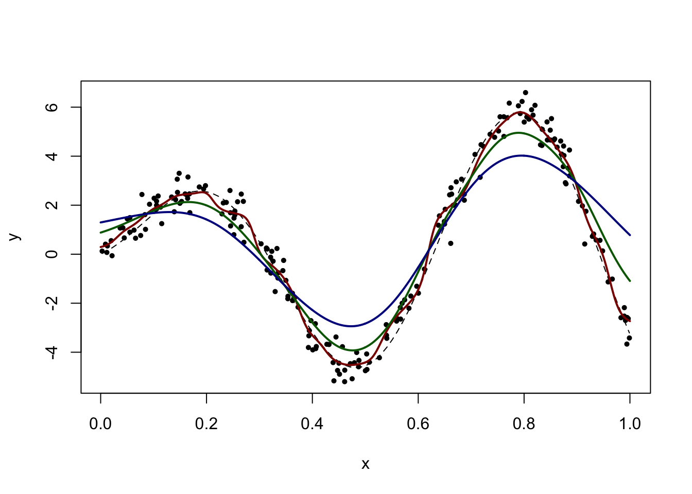

21.1.2 Choice of bandwidth by cross-validation

With a visual exploration, a choice of bandwidth around \(h = 0.05\) seems best. We now use cross-validation to choose the bandwidth to optimize prediction. Monte Carlo leave-k-out cross-validation is particularly easy to implement.

h_grid = seq(0.005, 0.1, len = 20) # grid of bandwidth values
m = round(n/10) # size of test set
B = 1e2 # number of monte carlo replicates
pred_error = matrix(NA, 20, B) # stores the prediction error estimates
for (k in 1:20) {
  h = h_grid[k]
  for (b in 1:B) {
    test = sort(sample(1:n, m))
    fit = ksmooth(x[-test], y[-test], x.points = x[test], "normal", bandwidth = h)
    pred_error[k, b] = sum((fit$y - y[test])^2)
  }
}
pred_error = apply(pred_error, 1, mean)
plot(h_grid, pred_error, type = "b", pch = 15, lwd = 2, xlab = "bandwidth", ylab = "estimated prediction error")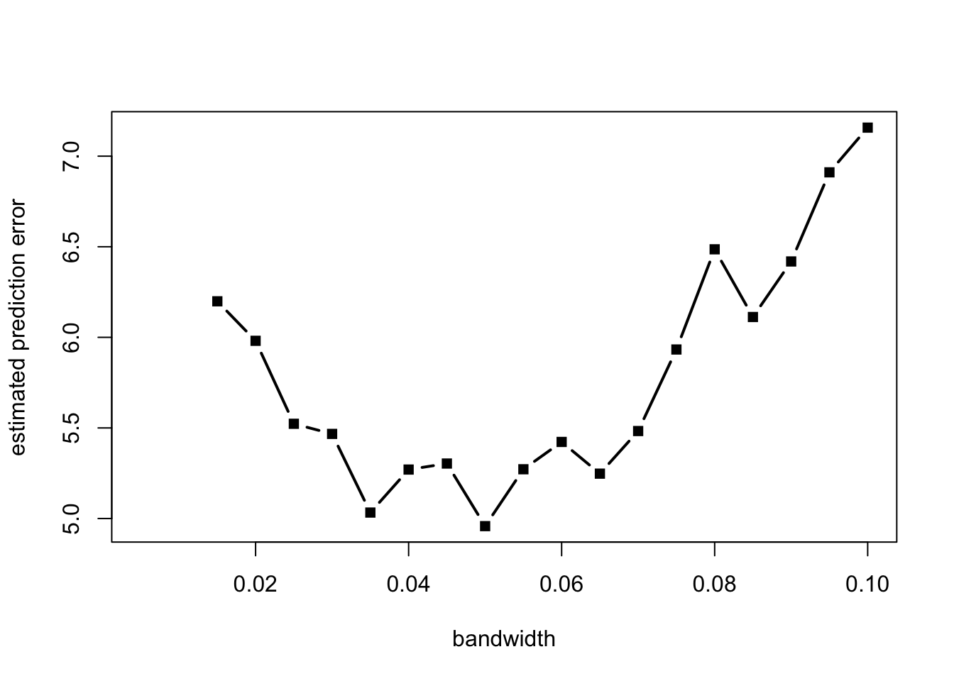

(h = h_grid[which.min(pred_error)])

[1] 0.05

plot_reset()
fit = ksmooth(x, y, "normal", bandwidth = h, x.points = x_new) # corresponding fit
lines(x_new, fit$y, col = "darkblue", lwd = 2)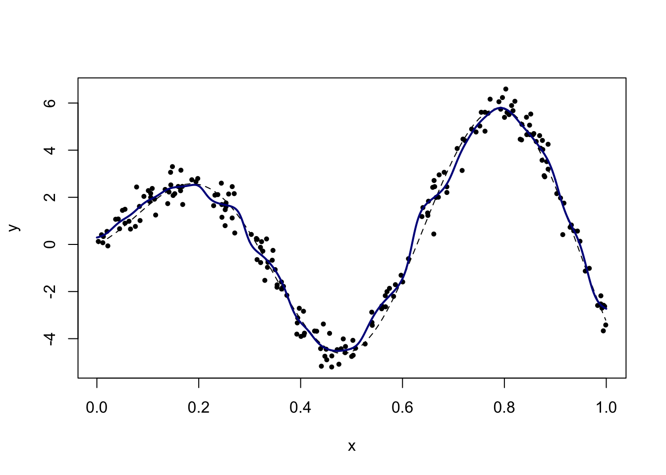

21.1.3 Local linear regression

require(KernSmooth)

We apply local linear regression and local cubic regression, after some visual exploration for the choice of bandwidth.

plot_reset()
fit = locpoly(x, y, bandwidth = 0.02)
lines(fit, col = "darkblue", lwd = 2)
fit = locpoly(x, y, degree = 3, bandwidth = 0.04)
lines(fit, col = "darkgreen", lwd = 2)
legend("topleft", legend = c("local linear", "local cubic"), col = c("darkblue", "darkgreen"), lty = 1, lwd = 2)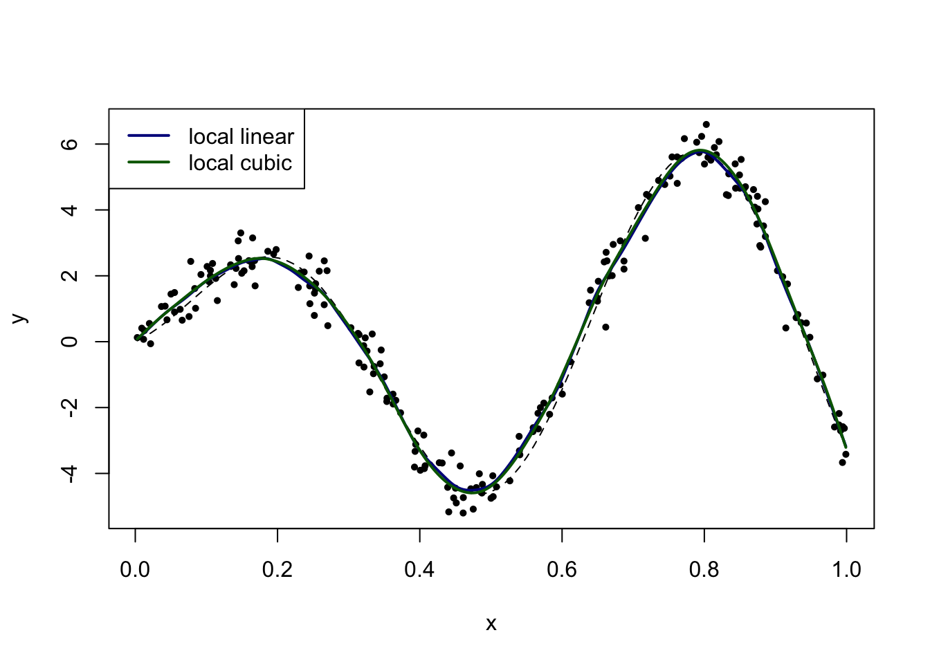

(In principle, we would perform cross-validation to select the bandwidth, but the function as implemented in this package can only be evaluated on a regular grid. (The function loess in the MASS package is another option, but it presents its own challenges.)

21.1.4 Polynomial regression

We now fit a polynomial model of varying degree. This is done using the lm function, which fits linear models (and polynomial models are linear models) according to the least squares criterion.

plot_reset()
for (d in 1:10) {
  fit = lm(y ~ poly(x, degree = d))
  lines(x, fit$fitted, lwd = 2, col = heat.colors(10)[d])
}

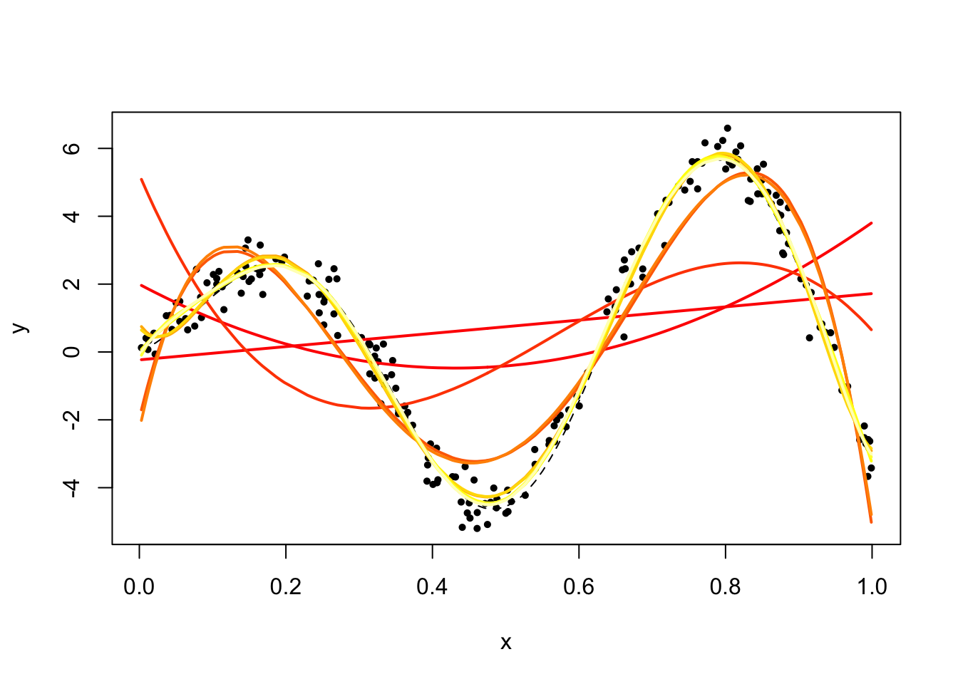
The fit at degree between 6 and 10 is quite good (even though the underlying function \(f\) is not a polynomial).

21.2 Classification

We consider the following synthetic dataset

n = 2000 # sample size
x1 = runif(n) # first predictor variable
x2 = runif(n) # second predictor variable
x = cbind(x1, x2)
y = as.numeric((x1-0.5)^2 + (x2-0.5)^2 <= 0.09) # response variable (two classes)
plot(x1, x2, pch = 16, col = y+2, asp = 1, xlab = "", ylab = "")
rect(0, 0, 1, 1, lty = 3)
require(plotrix)
draw.circle(0.5, 0.5, 0.3, lty = 2, lwd = 2)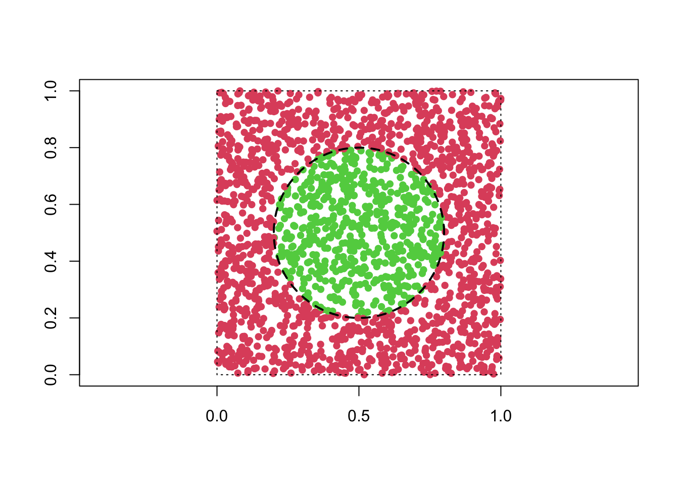

21.2.1 Nearest neighbor classifier

Nearest neighbor majority voting is readily available. (\(k\) below denotes the number of neighbors.)

require(class)
m = 50 
x_new = (1/m) * cbind(rep(1:m, m), gl(m, m)) # gridpoints
par(mfrow = c(2, 2), mai = c(0, 0, 0.2, 0))
class_color = c("white", "grey")
for (k in c(1, 3, 7, 10)) {
  val = knn(x, x_new, y, k = k)
  val = as.numeric(as.character(val))
  plot(x_new[, 1], x_new[, 2], pch = 15, col = class_color[val+1], asp = 1, xlab = "", ylab = "", main = paste("number of neighbors:", k), axes = FALSE)
  draw.circle(0.5, 0.5, 0.3, lty = 2, lwd = 2)
}

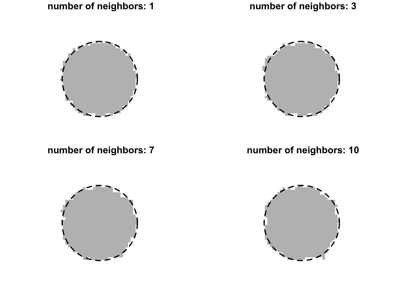
The classifier does not seem very sensitive to the choice of the number of nearest neighbors. Nevertheless, we can of course apply cross-validation to choose that parameter. The following implements leave-one-out cross-validation.

k_max = 30 # maximum number of neighbors
pred_error = numeric(k_max)
for (k in 1:k_max) {
  fit = knn.cv(x, y, k = k)
  pred_error[k] = sum(fit != y)
}
plot(1:k_max, pred_error, type = "b", pch = 15, lwd = 2, xlab = "number of neighbors", ylab = "estimated prediction error", axes = FALSE)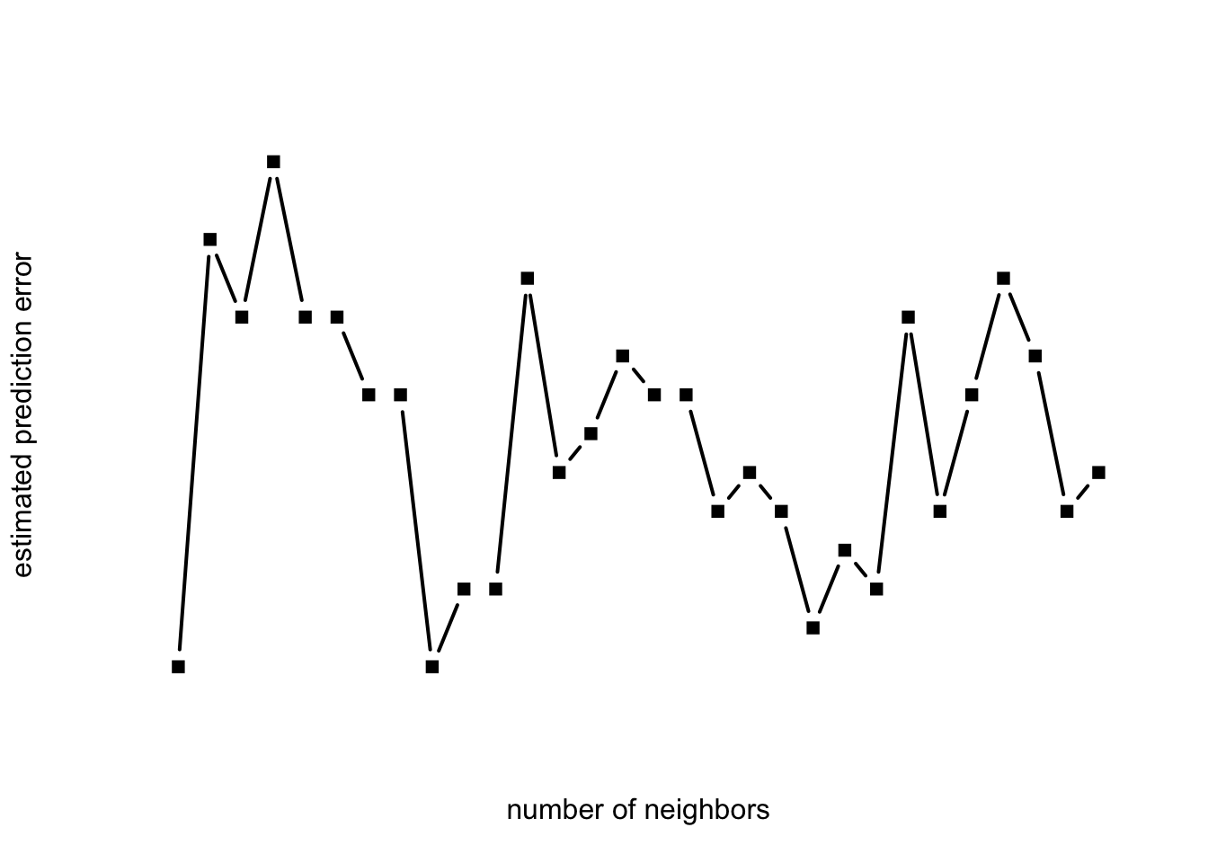

which.min(pred_error) 

[1] 1

The selected value of the parameters (number of neighbors) varies substantially from simulation to simulation, likely due to the fact that the sample size is relatively small and the performance is not very sensitive to the choice of parameter \(k\) within a certain range. (This sort of stability is typically considered a good thing.)

21.2.2 Linear classification

We first apply logistic regression based on a polynomial of degree 2 in the predictor variable(s). The fit is excellent (as expected).

dat = data.frame(x1 = x[, 1], x2 = x[, 2], y = y)
x_new = data.frame(x1 = x_new[, 1], x2 = x_new[, 2])
fit = glm(y ~ x1 + x2 + x1*x2 + I(x1^2) + I(x2^2), data = dat, family = "binomial")
prob = predict(fit, x_new, type = "response") # estimated probabilities
val = round(prob) # estimated classes
par(mai = c(0, 0, 0, 0))
plot(x_new[, 1], x_new[, 2], pch = 15, col = class_color[val+1], asp = 1, xlab = "", ylab = "", axes = FALSE)
draw.circle(0.5, 0.5, 0.3, lty = 2, lwd = 2)

We now turn to support vector machines with a polynomial kernel of degree 2. The fit is excellent (as expected).

require(kernlab)
dat$y = as.factor(dat$y)
fit = ksvm(y ~ ., data = dat, kernel = "polydot", kpar = list(degree = 2))
val = predict(fit, x_new, type = "response")
val = as.numeric(as.character(val))
par(mai = c(0, 0, 0, 0))
plot(x_new[, 1], x_new[, 2], pch = 15, col = class_color[val+1], asp = 1, xlab = "", ylab = "")
draw.circle(0.5, 0.5, 0.3, lty = 2, lwd = 2)