13 Properties of Estimators and Tests

13.1 Comparing estimators

A normal distribution is symmetric about its mean, so that its mean and median coincide. The question therefore arises: Should we use the sample mean or the sample median to estimate that parameter? Both seem equally natural, but the mean corresponds to the maximum likelihood estimator (MLE). We can run some simulations to compare these estimators. And indeed, the sample mean is somewhat better than the sample median, at least in terms of mean squared error, which is the performance measure that we use here.

q = 10
n_grid = 2^(1:q) # sample sizes
B = 1e3 # replicates
mean_error = numeric(q)
median_error = numeric(q)
for (k in 1:q) {
  n = n_grid[k]
  mean_out = numeric(B)
  median_out = numeric(B)
  for (b in 1:B) {
    x = rnorm(n) # normal sample
    mean_out[b] = mean(x) # sample mean 
    median_out[b] = median(x) # sample median 
  }
  mean_error[k] = mean(mean_out^2) # MSE for the sample mean 
  median_error[k] = mean(median_out^2) # MSE for the sample median
}
matplot(n_grid, cbind(mean_error, median_error), log = "xy", type = "b", lty = 1, pch = 15, lwd = 2, col = 2:3, xlab = "sample size", ylab = "mean squared error")
legend("topright", legend = c("sample mean", "sample median"), lty = 1, pch = 15, lwd = 2, col = 2:3)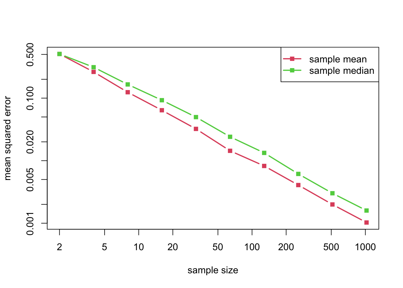

If instead of considering a normal distribution we consider a double-exponential distribution, the situation is exactly reversed.

q = 10
n_grid = 2^(1:q) # sample sizes
B = 1e3 # replicates
mean_error = numeric(q)
median_error = numeric(q)
for (k in 1:q) {
  n = n_grid[k]
  mean_out = numeric(B)
  median_out = numeric(B)
  for (b in 1:B) {
    x = rexp(n)*sample(c(-1,1), n, TRUE) # sample
    mean_out[b] = mean(x) # double-exponential sample mean 
    median_out[b] = median(x) # sample median 
  }
  mean_error[k] = mean(mean_out^2) # MSE for the sample mean 
  median_error[k] = mean(median_out^2) # MSE for the sample median
}
matplot(n_grid, cbind(mean_error, median_error), log = "xy", type = "b", lty = 1, pch = 15, lwd = 2, col = 2:3, xlab = "sample size", ylab = "(estimated) mean squared error")
legend("topright", legend = c("sample mean", "sample median"), lty = 1, pch = 15, lwd = 2, col = 2:3)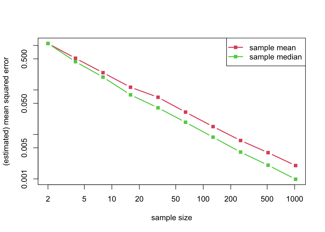

13.2 Uniformly most powerful tests

Consider testing \(Q_0\) versus \(Q_1\), two distributions on the same discrete space. The Neyman–Pearson Lemma implies that a likelihood ratio test (LRT) is most powerful at the level equal to its size. In turn, computing an LRT in the present setting involves solving an integer program. Below, we generate two random distributions on \(\{1, \dots, 10\}\), and then solve the integer program defining the LRT at level \(\alpha = 0.20\).

Q0 = runif(10)
Q0 = Q0/sum(Q0)
Q1 = runif(10)
Q1 = Q1/sum(Q1)
LR = Q1/Q0

require(lpSolve)
alpha = 0.20
Objective = Q1
Constraint = t(as.matrix(Q0))
L = lp("max", Objective, Constraint, "<=", alpha, all.bin = TRUE)
reject = which(L$solution == 1)

The rejection region is

cat(reject)

2 4 5

The size of the test is the probability of rejecting under the null, that is, the probability of the rejection region under \(Q_0\)

sum(Q0[reject])

[1] 0.1519911

It is upper-bounded by the level by design.