7 Expectation and Concentration

7.1 Concentration inequalities

Let us compare the accuracy of some of the main concentration inequalities in the example of a binomial distribution. We consider \(Y\) to be binomial with parameters \((n, p)\) specified below, and compute the bounds given by Markov, Chebyshev, Bernstein, and Chernoff, which we then compare visually in several ways.

n = 30 # size parameter
p = 0.2 # probability parameter
mu = n*p # mean
sigma = sqrt(n*p*(1-p)) # standard deviation
y = ceiling(mu):n # possible values above the mean

Markov’s upper bound:

markov = mu/y

Chebyshev’s upper bound:

chebyshev = 1/(1 + (y-mu)^2/sigma^2)

Bernstein’s upper bound:

bernstein = exp(- ((y-mu)^2/2)/(sigma^2 + (y-mu)/3))

Chernoff’s upper bound:

b = y/n
chernoff = exp(- n*(b*log(b/p) + (1-b)*log((1-b)/(1-p))))
chernoff[length(chernoff)] = exp(- n*log(1/p)) # the second term in the exponential is 0 by convention when b = 1

Exact upper tail:

exact = pbinom(y-1, n, p, lower.tail = FALSE)

First, we plot the bounds

matplot(y, cbind(markov, chebyshev, bernstein, chernoff, exact), type = "b", lty = 1, lwd = 2, pch = 15, xlab = "", ylab = "upper tail", col = grey((4:0)/5))
legend("topright", legend = c("markov", "chebyshev", "bernstein", "chernoff", "exact"), lty = 1, lwd = 2, pch = 15, col = grey((4:0)/5))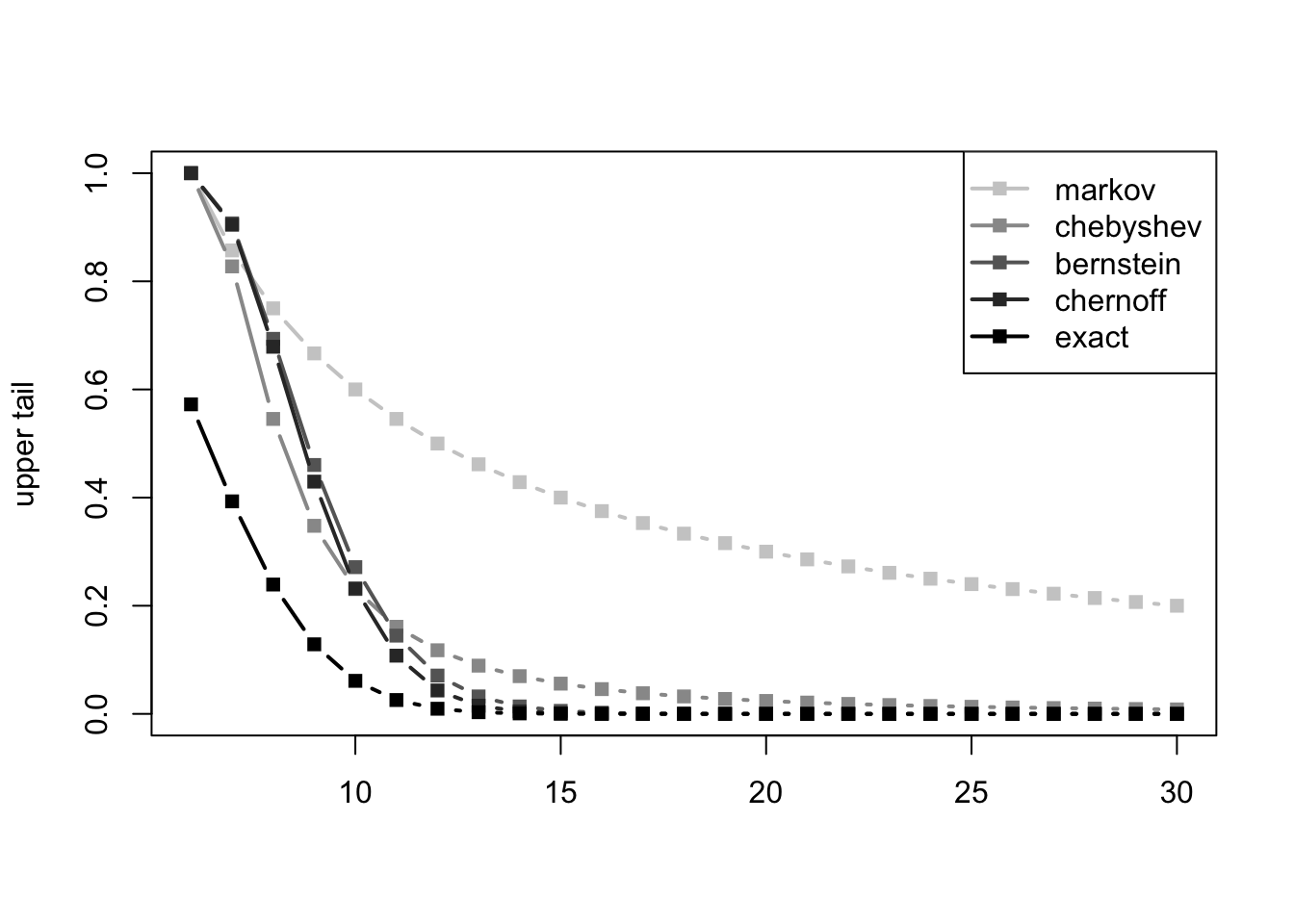

Next, we plot the ratios of the bounds to the exact value. We do it in a logarithmic scale as some of the bounds are orders of maginture more accurate than others.

matplot(y, log(cbind(markov, chebyshev, bernstein, chernoff, exact)/exact), type = "b", lty = 1, lwd = 2, pch = 15, xlab = "", ylab = "upper tail ratio", col = grey((4:0)/5))
legend("topleft", legend = c("markov", "chebyshev", "bernstein", "chernoff", "exact"), lty = 1, lwd = 2, pch = 15, col = grey((4:0)/5))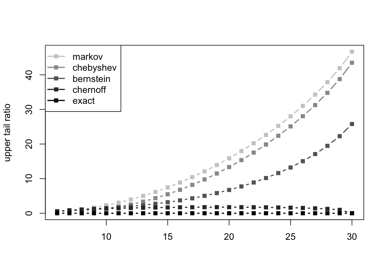

Even though Chernoff’s bound is orders of magnitude more accurate than the other bounds (this is true here and can be proven to be true in general), the other bounds remain useful, trading accuracy for simplicity.