4 Discrete Distributions

4.1 Uniform distributions

Consider the uniform distribution on \(\{0, \dots, n\}\) with

n = 20

Its mass function (when defined on the integers) is given by

dunid = function(k, n) (n+1)^{-1}*(0 <= k)*(k <= n)

Here is a graph of this function

k = -3:(n+3)
plot(k, dunid(k, n), type = "h", lwd = 2, xlab = "", ylab = "")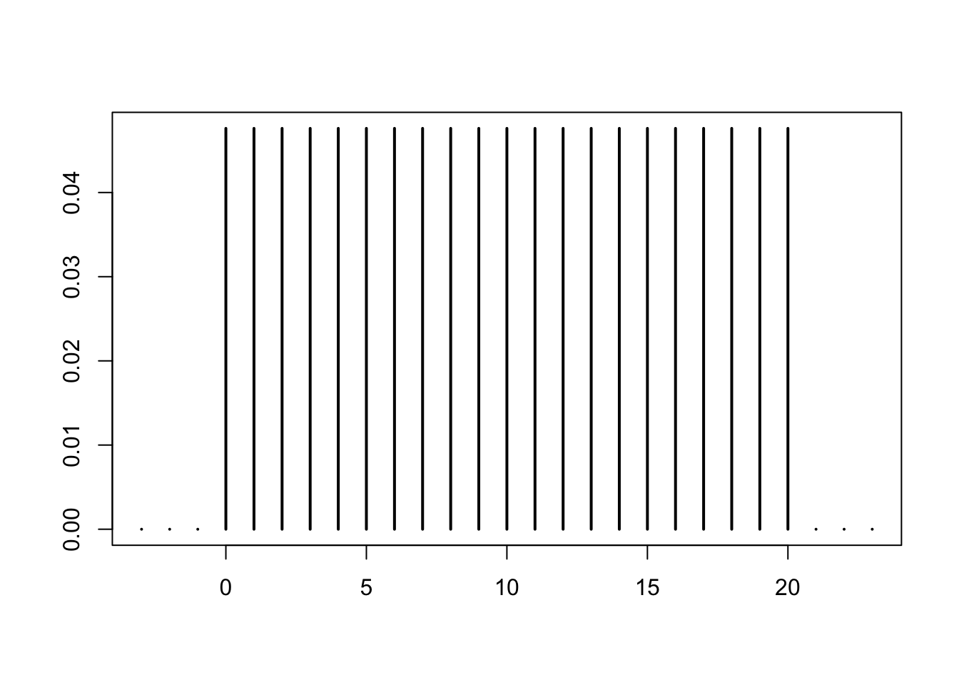

Its distribution function (when defined on the reals) is given by

punid = function(x, n) pmin(1, pmax(0, floor(x+1))/(n+1))

Here is a graph of this function

curve(punid(x, n), -3, n+3, 1e3, lwd = 2, xlab = "", ylab = "")
abline(h = c(0, 1), lty = 2)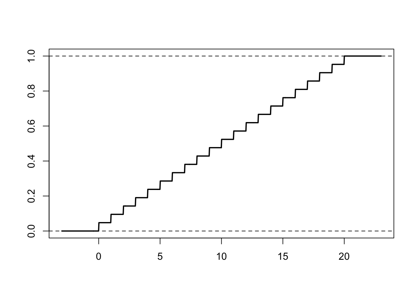

4.2 Binomial distributions

Consider the binomial distribution with the following parameters

n = 20
p = 0.2

Here is a plot of its mass function

k = -3:(n+3)
plot(k, dbinom(k, n, p), type = "h", lwd = 2, xlab = "", ylab = "")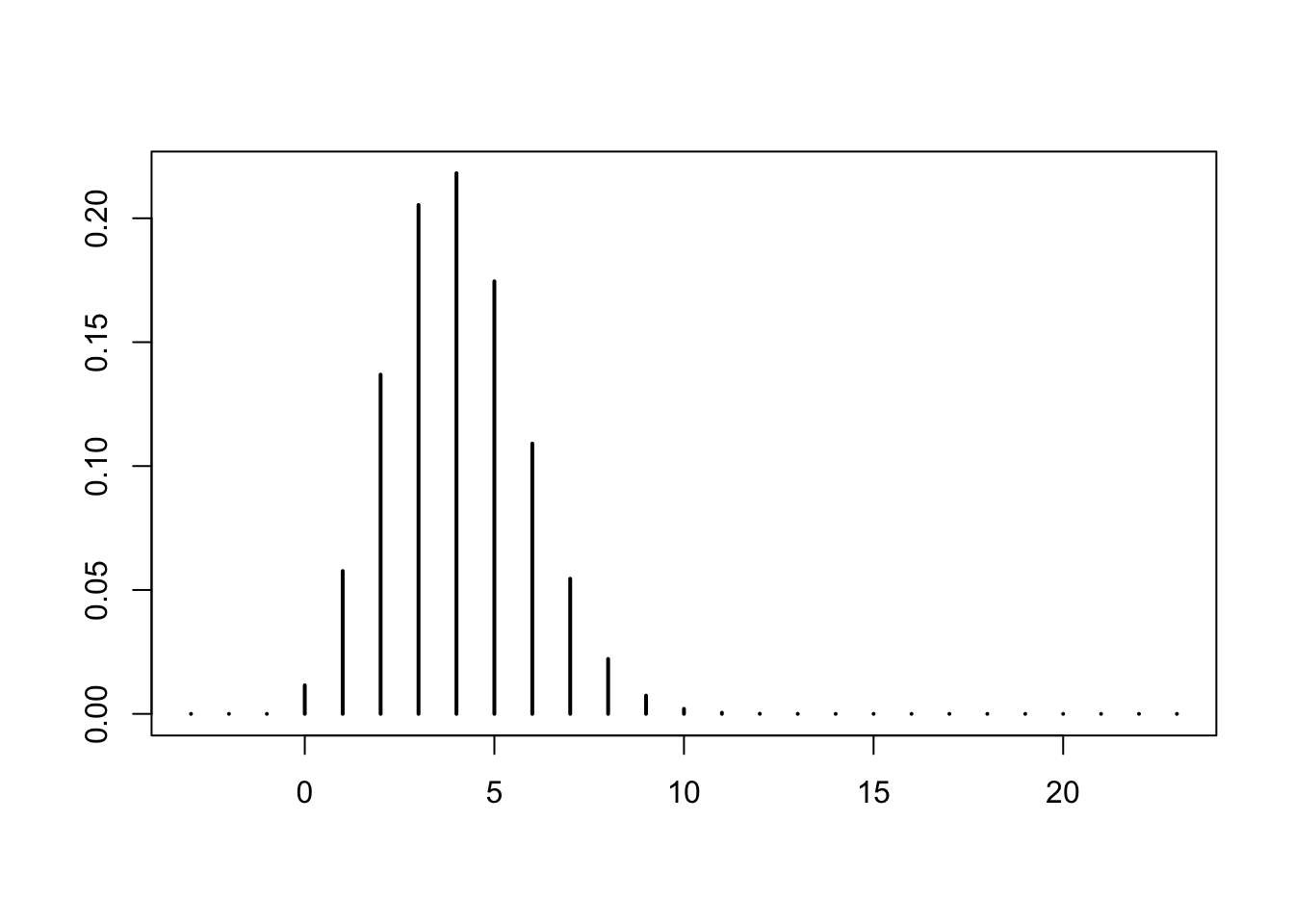

Here is a plot of its (cumulative) distribution function

curve(pbinom(x, n, p), -3, n+3, 1e3, lwd = 2, xlab = "", ylab = "")
abline(h = c(0, 1), lty = 2)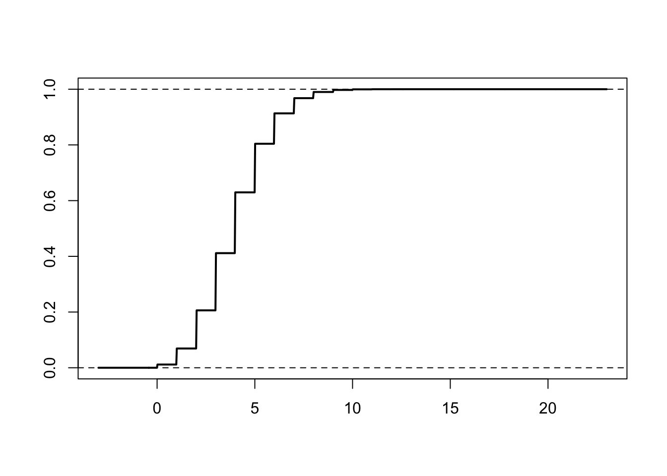

4.3 Geometric distributions

Consider the geometric distribution with the following parameter

p = 0.2

Here is a plot of its mass function

k = -3:30
plot(k, dgeom(k, p), type = "h", lwd = 2, xlab = "", ylab = "")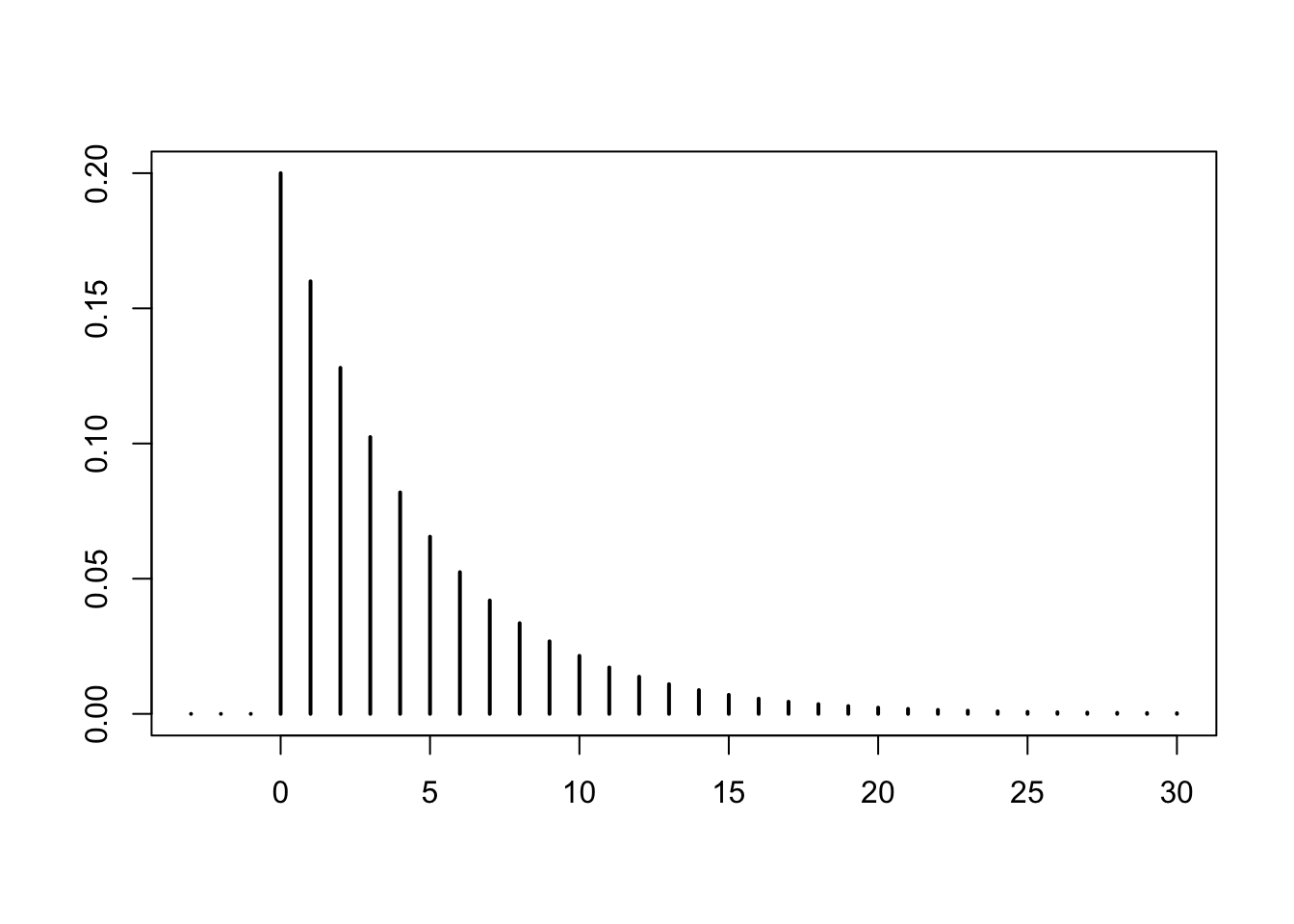

Here is a plot of its (cumulative) distribution function

curve(pgeom(x, p), -1, 30, 1e3, lwd = 2, xlab = "", ylab = "")
abline(h = c(0, 1), lty = 2)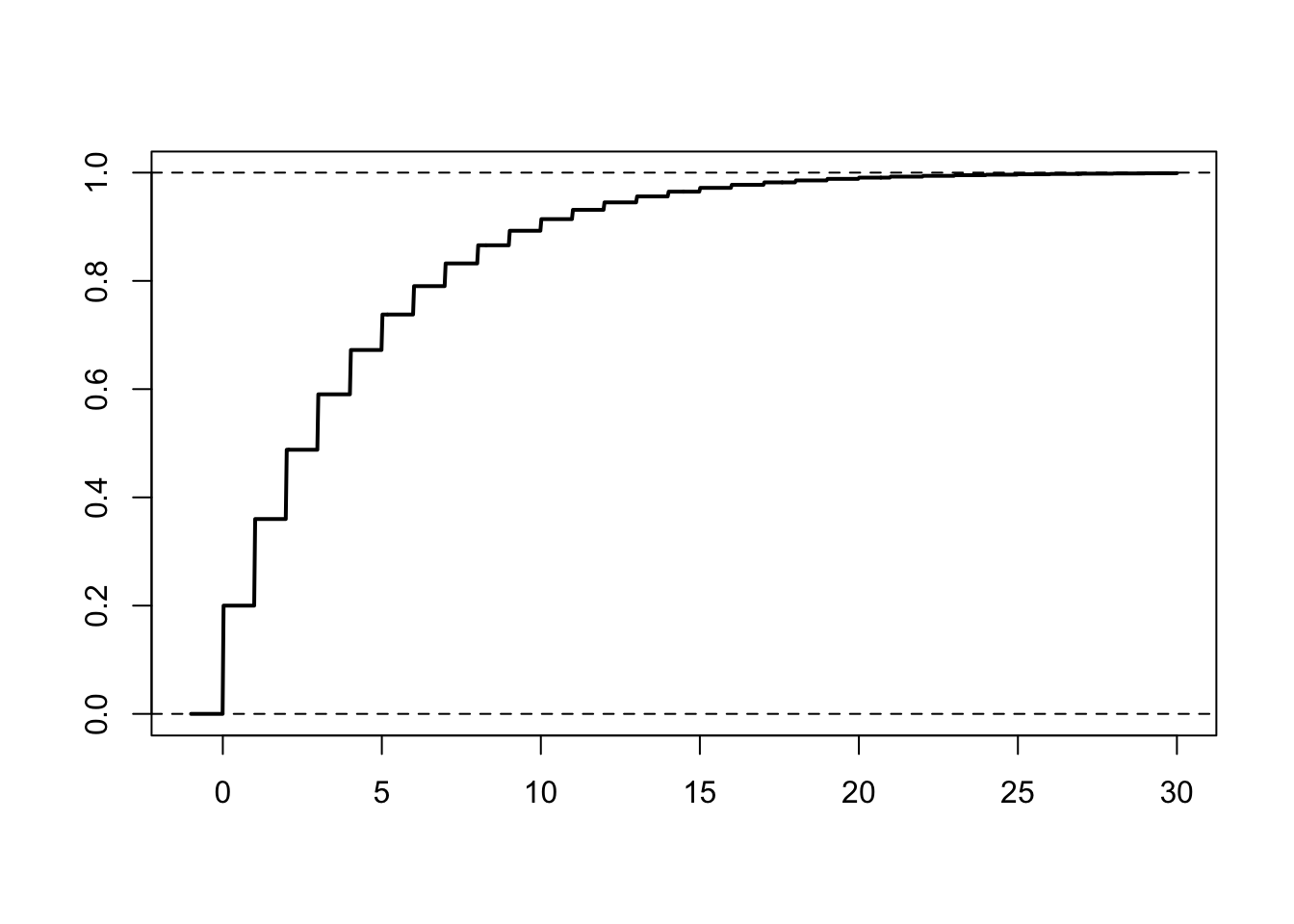

4.4 Poisson distributions

Consider the Poisson distribution with the following parameter

lambda = 5

Here is a plot of its mass function

k = -3:30
plot(k, dpois(k, lambda), type = "h", lwd = 2, xlab = "", ylab = "")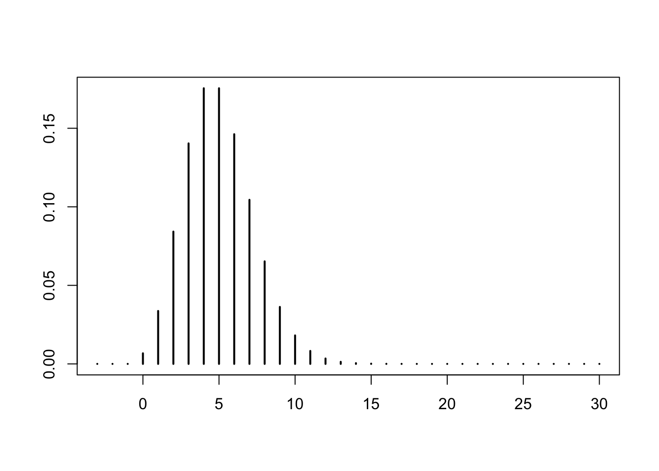

Here is a plot of its (cumulative) distribution function

curve(ppois(x, lambda), -1, 30, 1e3, lwd = 2, xlab = "", ylab = "")
abline(h = c(0, 1), lty = 2)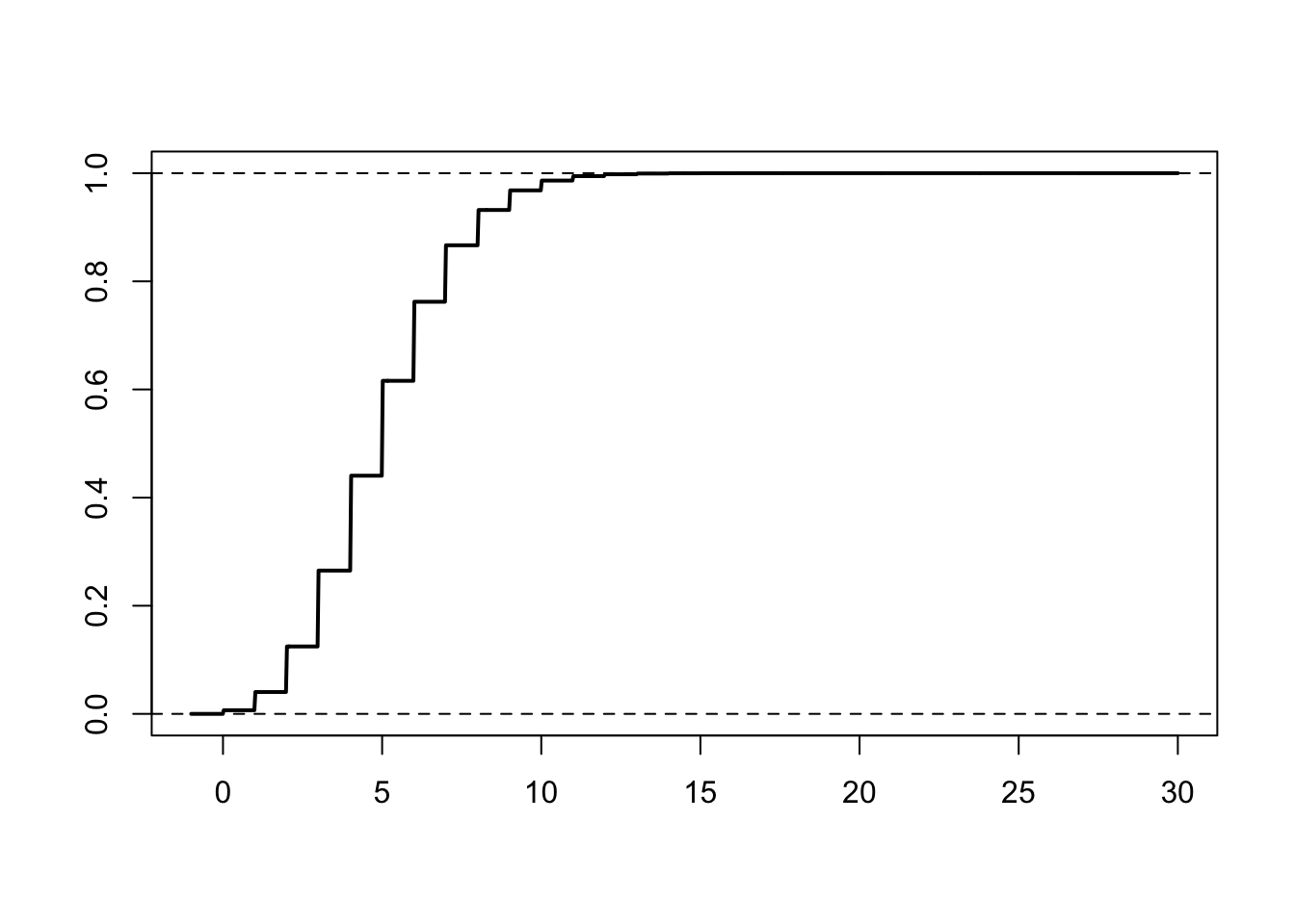

Let’s check the validity of the Law of Small Numbers. We work with the following parameters

n = 100
p = 2/n
lambda = n*p
k = 0:10 # focusing on the interesting area

We first compare the mass functions (the horizontal offset is for plotting purposes only)

plot(c(k, k+0.1), c(dbinom(k, n, p), dpois(k, lambda)), type = "h", lwd = 2, xlab = "", ylab = "", col = c(rep("darkgreen", length(k)), rep("darkblue", length(k))))
legend("topright", c("binomial", "Poisson"), lty = 1, lwd = 2, col = c("darkgreen", "darkblue"))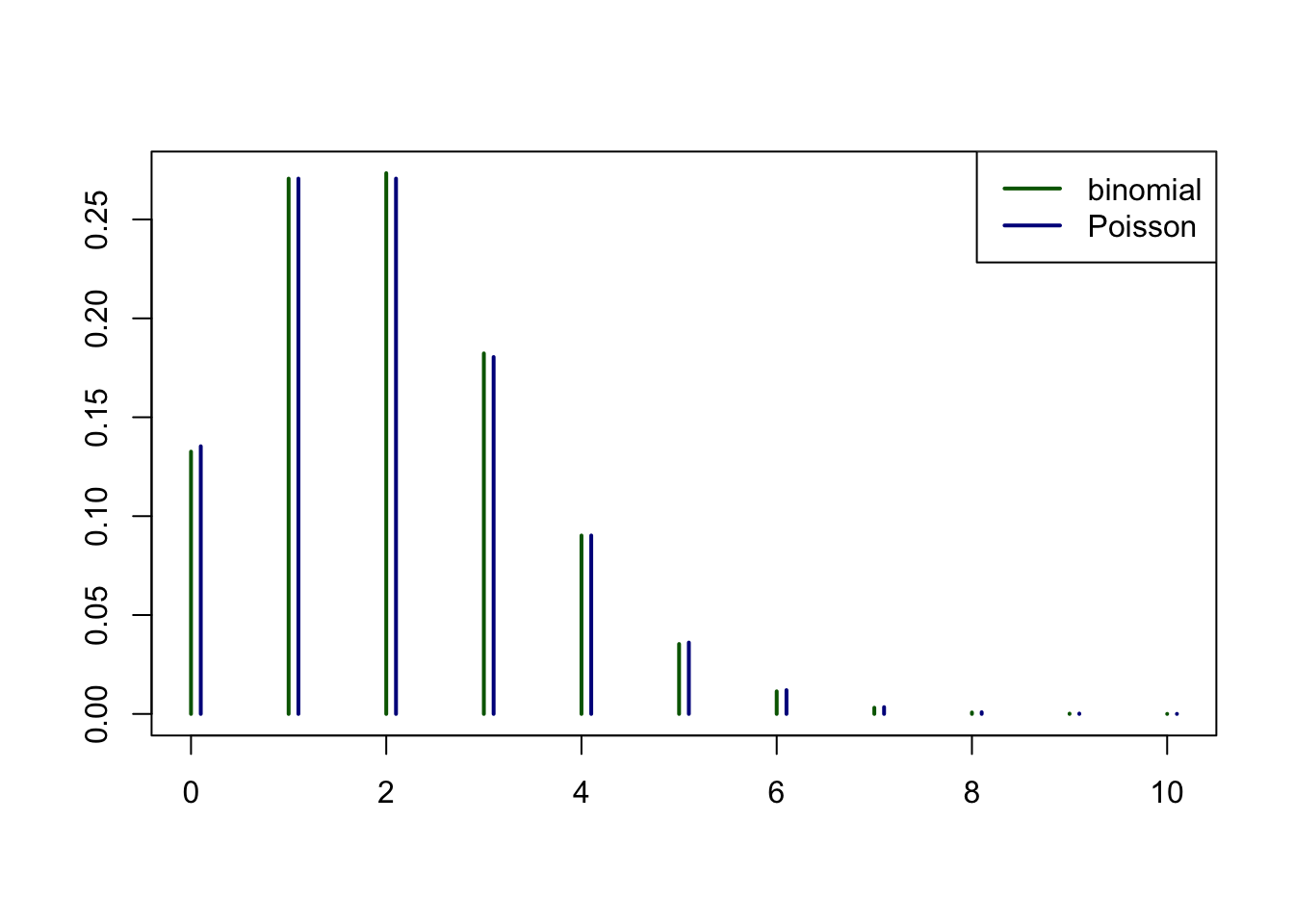

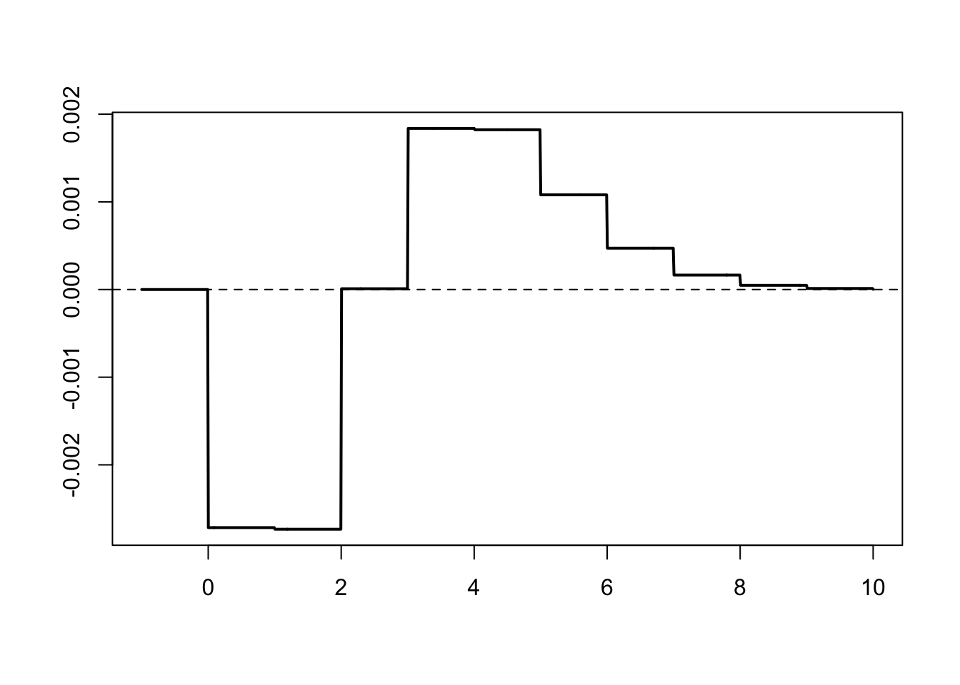
Better yet, we plot the difference in absolute value (notice the range on the vertical axis)

plot(k, dbinom(k, n, p) - dpois(k, lambda), type = "h", lwd = 2, xlab = "", ylab = "")
abline(h = 0, lty = 2)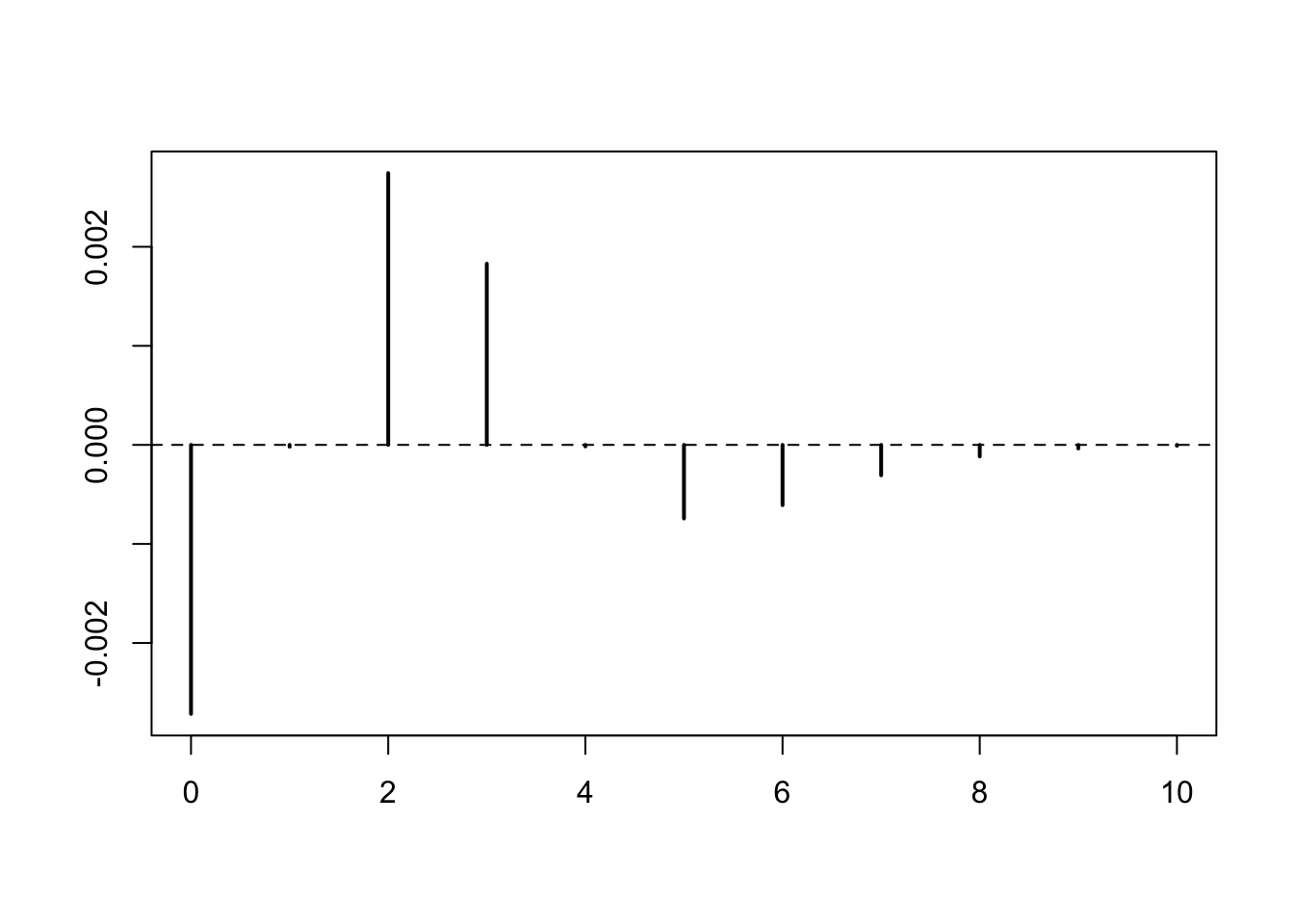

We now compare the (cumulative) distribution functions

curve(pbinom(x, n, p), -1, 10, 1e3, lwd = 2, xlab = "", ylab = "", col = "darkgreen")
curve(ppois(x, lambda), -1, 10, 1e3, lwd = 2, add = TRUE, col = "darkblue")
abline(h = c(0, 1), lty = 2)
legend("bottomright", c("binomial", "Poisson"), lty = 1, lwd = 2, col = c("darkgreen", "darkblue"))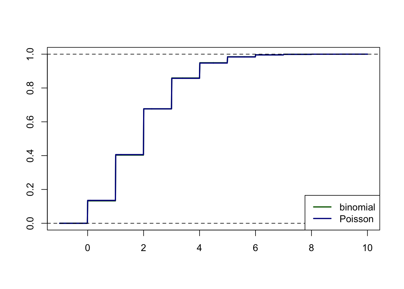

As these curves are almost indistinguishable (second confirmation that the approximation is very good), we plot the difference

curve(pbinom(x, n, p) - ppois(x, lambda), -1, 10, 1e3, lwd = 2, xlab = "", ylab = "")
abline(h = 0, lty = 2)