Chapter 13 Missing data
13.1 Objectives
At the end of the chapter, readers will be able to:
- To perform a simple imputation
- To perform a single imputation
- To perform a multiple imputation
13.2 Introduction
Missing data can significantly affect the performance of predictive risk modeling, an important technique for developing medical guidelines. The two most commonly used strategies for managing missing data are to impute or delete values, and the former can cause bias, while the later can cause both bias and loss of statistical power. Several techniques designed to deal with missing data are described and applied to an illustrative example. These methods include complete-case analysis, available-case analysis, as well as single and multiple imputation.
Researchers should report the details of missing data, and appropriate methods for dealing with missing values should be incorporated into the data analysis.
13.3 Types of missing data
Missing data data is quite a common issue in research. The causes of missing data should always be investigated and more data should be collected if possible. There are three types of missing data:
- Missing completely at random (MCAR)
- Missing at random (MAR)
- Missing not at random (MNAR)
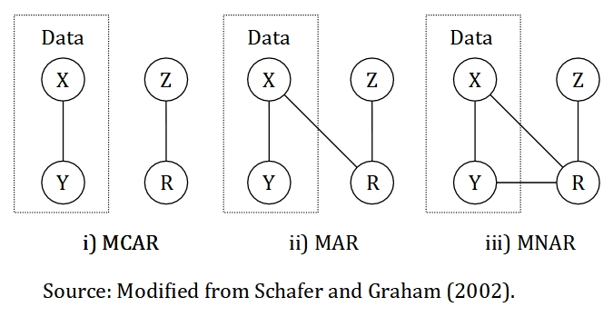
FIGURE 13.1: Illustration of missing data mechanism for the three types of missing data. The data is made up of X and Y. X represents a variable with completely observed values, Y represents a variable with missing values, Z represents a cause of missing values and R represents an indicator variable that identify missing and observed values in Y, in other words, the missingness.
Missing data is classified as MCAR if the missingness is unrelated to the data. For example, medical records that is lost due to flood and laboratory equipment malfunction, Z. In other words, the data is missing totally by chance. We can relate this example to the Figure 13.1, the missingness, R is not related to the data itself, which is a combination of variables with completely observed values, X and variables with partly missing values, Y. MCAR is ideal and more convenient, though MAR is more common and realistic.
Missing data is said to be MAR if the missingness is related to other values that we completely observed, but not to the variable with missing values itself. For example, an older person is more likely to complete a survey compared to the younger person. So, the missingness is related to age, a variable that has been observed in the data. Similarly, if information on income is more likely to be missing for older individuals as they are more cautious to reveal a sensitive information as opposed to younger individuals. Thus, the missingness is related to age, which should be a variable that we have collected during the survey. The similarity of the two examples is that we completely observed the variable age. Another example of MAR is missing a certain variable due to the old medical form do not include this information in the form. However, a new updated medical form include this information. As the missingness is not related to the variable with missing values itself and we have the information whether the patients use an old or a new medical form, we can classify this missingness as MAR. We can see from all the examples that the missingness, R is related to other variables that we completely observed, X, but not to the variable with missing values itself, Y as illustrated in the Figure 13.1.
Lastly, the missing data is considered MNAR if the missingness is related to the variable with missing values itself and other variables with completely observed values as well. Also, the missingness is considered MNAR if the causes completely unknown to us. In other words, we can not logically deduce that the missing data fit MCAR or MAR types. For example, missing a weight information for an obese individuals as the normal weighing scale may not able to weigh the individuals. Thus, according to 13.1, the pattern of missingness is considered MNAR as the missingness, R is related the variable with partly missing values itself, Y. However, we can never be sure of this without a further investigation about the mechanism of missingness and its causes. MNAR is the most problematic type among the three. There are a few approaches to differentiate between MCAR and MAR-MNAR. However, an approach to differentiate between MAR and MNAR has yet to be proposed. Thus, we need to use a logical reasoning to differentiate between the two types.
Alternatively, Figure 13.1 can be represented mathematically as follows:
\[MCAR: P(R|Z)\] \[MAR: P(R|X,Z)\] \[MNAR: P(R|X,Y,Z)\] In MCAR, the missingness is completely related to the cause of missing data, Z, which is unrelated to variables with completely observed values, X and variables with missing values, Y. However, MAR allows the missingness to be related to X, on top of Z. Additionally, MNAR requires the missingness related to X, Y, and Z.
13.4 Preliminaries
13.4.1 Packages
We will use these packages:
- mice: for the single and multiple imputation
- VIM: for missing data exploration
- naniar: for missing data exploration
- tidyverse: for data wrangling and manipulation
- gtsummary: to provide a nice result in a table
library(mice)
library(VIM)
library(naniar)
library(tidyverse)
library(gtsummary)
13.4.2 Dataset
We going to use the coronary dataset that we used previously in linear regression chapter. However, this dataset have been altered to generate a missing values in it.
coroNA <- read_csv(here::here('data', "coronaryNA.csv"))Next, we going to transform the all the character variables into a factor. mutate_if() will recognise all character variables and transform it into a factor.
coroNA <-
  coroNA %>%
  mutate_if(is.character, as.factor)
summary(coroNA)
## age race chol id cad
## Min. :33.00 chinese:31 Min. :4.000 Min. : 1.0 cad : 37
## 1st Qu.:43.00 indian :45 1st Qu.:5.362 1st Qu.: 901.5 no cad:163
## Median :48.00 malay :49 Median :6.050 Median :2243.5
## Mean :48.02 NA's :75 Mean :6.114 Mean :2218.3
## 3rd Qu.:53.00 3rd Qu.:6.875 3rd Qu.:3346.8
## Max. :62.00 Max. :9.350 Max. :4696.0
## NA's :85 NA's :33
## sbp dbp bmi gender
## Min. : 88.0 Min. : 56.00 Min. :28.99 man :100
## 1st Qu.:115.0 1st Qu.: 72.00 1st Qu.:36.10 woman:100
## Median :126.0 Median : 80.00 Median :37.80
## Mean :130.2 Mean : 82.31 Mean :37.45
## 3rd Qu.:144.0 3rd Qu.: 92.00 3rd Qu.:39.20
## Max. :187.0 Max. :120.00 Max. :45.03
## Missing data in R is denoted by NA. Further information about NA can be assessed by typing ?NA in the RStudio console. As seen above, the three variables; age, race and chol have missing values. We can further confirm this using a anyNA().
anyNA(coroNA)## [1] TRUETrue indicates a presence of missing values in our data. Thus, we can further explore the missing values in our data.
13.5 Exploring missing data
The total percentage of missing values in our data is 10.7%.
prop_miss(coroNA)## [1] 0.1072222Percentage of missing data by variable:
miss_var_summary(coroNA)## # A tibble: 9 × 3
## variable n_miss pct_miss
## <chr> <int> <dbl>
## 1 age 85 42.5
## 2 race 75 37.5
## 3 chol 33 16.5
## 4 id 0 0
## 5 cad 0 0
## 6 sbp 0 0
## 7 dbp 0 0
## 8 bmi 0 0
## 9 gender 0 0Both prop_miss() and miss_var_summary() are from naniar package. Subsequently, We can explore the pattern of missing data using aggr() function from VIM. The numbers and prop arguments indicate that we want the missing information on the y-axis of the plot to be in number not proportion.
aggr(coroNA, numbers = TRUE, prop = FALSE)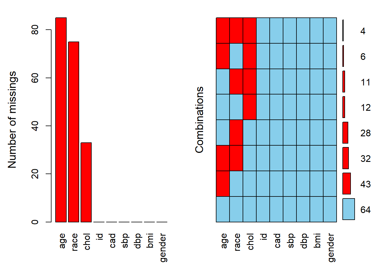
The labels on x-axis are according to the column names in the dataset. In term of pattern of missingness, about 43 observation are missing age values alone.
Similarly, the pattern of missing data can be explore through md.pattern() from mice package. The rotate.names argument set to true to specify the direction of the variable names on top of the plot horizontally.
md.pattern(coroNA, rotate.names = TRUE)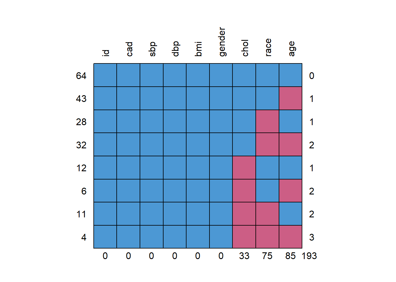
##    id cad sbp dbp bmi gender chol race age
## 64  1   1   1   1   1      1    1    1   1   0
## 43  1   1   1   1   1      1    1    1   0   1
## 28  1   1   1   1   1      1    1    0   1   1
## 32  1   1   1   1   1      1    1    0   0   2
## 12  1   1   1   1   1      1    0    1   1   1
## 6   1   1   1   1   1      1    0    1   0   2
## 11  1   1   1   1   1      1    0    0   1   2
## 4   1   1   1   1   1      1    0    0   0   3
##     0   0   0   0   0      0   33   75  85 193
Additionally, we can assess the correlation:
- Between variables with missing values
- Between variables with missing values and variable with non-missing values
First, we need to take variables with missing values only. Then, we code a missing value with 1 and non-missing value with 0.
dummyNA <-
  as.data.frame(abs(is.na(coroNA))) %>%
  select(age, race, chol) # pick variable with missing values only
head(dummyNA)
## age race chol
## 1 0 0 0
## 2 0 0 0
## 3 0 0 0
## 4 1 0 0
## 5 1 0 0
## 6 0 0 0We assess the correlation between variables with missing values.
cor(dummyNA) %>% round(digits = 2)## age race chol
## age 1.00 0.09 -0.11
## race 0.09 1.00 0.07
## chol -0.11 0.07 1.00There is no strong correlation between variables with missing values. We can conclude that the missing values in one variable is not related to the missing values in another variable.
The second correlation is between variables with missing values and variable with non-missing values. First, we need to change the categorical variable into a numeric value to get a correlation for all the variables.
cor(coroNA %>% mutate_if(is.factor, as.numeric),
    dummyNA, use = "pairwise.complete.obs") %>%
  round(digits = 2)
## Warning in cor(coroNA %>% mutate_if(is.factor, as.numeric), dummyNA, use =
## "pairwise.complete.obs"): the standard deviation is zero## age race chol
## age NA 0.04 0.04
## race 0.02 NA 0.01
## chol -0.11 -0.06 NA
## id 0.01 -0.06 -0.07
## cad 0.02 0.05 -0.17
## sbp -0.07 0.04 0.17
## dbp -0.04 0.04 0.17
## bmi 0.13 -0.08 -0.76
## gender 0.07 0.03 -0.07We can safely ignore the warning generated in the result. Variables on the left side are variable with non-missing values and variables on the top of the columns are variables with missing values. There is a high correlation (-0.76) between bmi and chol indicating values of chol are more likely to be missing at lower values of bmi.
Lastly, we can do a Little’s test to determine if the missing data is MCAR or other types. The null hypothesis is the missing data is MCAR. Thus, a higher p value indicates probability of missing data is MCAR. The test shows that the missingness in our data is either MAR or MNAR.
mcar_test(coroNA)## # A tibble: 1 × 4
## statistic df p.value missing.patterns
## <dbl> <dbl> <dbl> <int>
## 1 158. 51 8.25e-13 813.6 Handling missing data
We going to cover four approaches to handling missing data:
- Listwise deletion
- Simple imputation:
- Mean substitution
- Median substitution
- Mode substitution
- Single imputation:
- Regression imputation
- Stochastic regression imputation
- Decision tree imputation
- Multiple imputation
Each approach has their own caveats which we will cover in each section below.
13.6.1 Listwise deletion
Listwise or case deletion is the default setting in R. By default, R will exclude all the rows with missing data.
lw <- lm(dbp ~ ., data = coroNA)
summary(lw)
##
## Call:
## lm(formula = dbp ~ ., data = coroNA)
##
## Residuals:
## Min 1Q Median 3Q Max
## -16.7770 -3.8094 -0.0874 3.5889 13.3479
##
## Coefficients:
## Estimate Std. Error t value Pr(>|t|)
## (Intercept) 34.6358468 20.5615343 1.684 0.0979 .
## age -0.2764718 0.2139740 -1.292 0.2018
## raceindian 4.6080430 2.9423909 1.566 0.1232
## racemalay -0.1318924 2.6075792 -0.051 0.9598
## chol 0.7174697 0.8142408 0.881 0.3821
## id 0.0000390 0.0006004 0.065 0.9484
## cadno cad -1.2884879 2.2026942 -0.585 0.5610
## sbp 0.5390141 0.0502732 10.722 5.48e-15 ***
## bmi -0.4189575 0.4086179 -1.025 0.3098
## genderwoman 2.3084961 1.6749082 1.378 0.1738
## ---
## Signif. codes: 0 '***' 0.001 '**' 0.01 '*' 0.05 '.' 0.1 ' ' 1
##
## Residual standard error: 6.218 on 54 degrees of freedom
## (136 observations deleted due to missingness)
## Multiple R-squared: 0.7581, Adjusted R-squared: 0.7177
## F-statistic: 18.8 on 9 and 54 DF, p-value: 1.05e-13As shown in the information above (at the bottom), 136 rows or observations were excluded due to missingness. Listwise deletion approach able to produce an unbiased result only when the missing data is MCAR and the amount of missing data is relatively small.
13.6.2 Simple imputation
A simple imputation includes mean, median and mode substitution is a relatively easy approach. In this approach, the missing values is replaced by a mean or median for numerical variable, and mode for categorical variable. This simple imputation approach only appropriate if missing data is MCAR and the amount of missing data is relatively small.
- Mean substitution
replace_na will replace the missing values in age with its mean.
mean_sub <-
  coroNA %>%
  mutate(age = replace_na(age, mean(age, na.rm = T)))

summary(mean_sub)
## age race chol id cad
## Min. :33.00 chinese:31 Min. :4.000 Min. : 1.0 cad : 37
## 1st Qu.:46.00 indian :45 1st Qu.:5.362 1st Qu.: 901.5 no cad:163
## Median :48.02 malay :49 Median :6.050 Median :2243.5
## Mean :48.02 NA's :75 Mean :6.114 Mean :2218.3
## 3rd Qu.:49.00 3rd Qu.:6.875 3rd Qu.:3346.8
## Max. :62.00 Max. :9.350 Max. :4696.0
## NA's :33
## sbp dbp bmi gender
## Min. : 88.0 Min. : 56.00 Min. :28.99 man :100
## 1st Qu.:115.0 1st Qu.: 72.00 1st Qu.:36.10 woman:100
## Median :126.0 Median : 80.00 Median :37.80
## Mean :130.2 Mean : 82.31 Mean :37.45
## 3rd Qu.:144.0 3rd Qu.: 92.00 3rd Qu.:39.20
## Max. :187.0 Max. :120.00 Max. :45.03
## - Median substitution
replace_na will replace the missing values in age with its median.
med_sub <-
  coroNA %>%
  mutate(age = replace_na(age, median(age, na.rm = T)))

summary(med_sub)
## age race chol id cad
## Min. :33.00 chinese:31 Min. :4.000 Min. : 1.0 cad : 37
## 1st Qu.:46.00 indian :45 1st Qu.:5.362 1st Qu.: 901.5 no cad:163
## Median :48.00 malay :49 Median :6.050 Median :2243.5
## Mean :48.01 NA's :75 Mean :6.114 Mean :2218.3
## 3rd Qu.:49.00 3rd Qu.:6.875 3rd Qu.:3346.8
## Max. :62.00 Max. :9.350 Max. :4696.0
## NA's :33
## sbp dbp bmi gender
## Min. : 88.0 Min. : 56.00 Min. :28.99 man :100
## 1st Qu.:115.0 1st Qu.: 72.00 1st Qu.:36.10 woman:100
## Median :126.0 Median : 80.00 Median :37.80
## Mean :130.2 Mean : 82.31 Mean :37.45
## 3rd Qu.:144.0 3rd Qu.: 92.00 3rd Qu.:39.20
## Max. :187.0 Max. :120.00 Max. :45.03
## - Mode substitution
We need to find the mode, the most frequent level or group in the variable. In race variable, it is malay.
table(coroNA$race)##
## chinese indian malay
## 31 45 49replace_na will replace the missing values in race with its mode.
mode_sub <-
  coroNA %>%
  mutate(race = replace_na(race, "malay"))

summary(mode_sub)
## age race chol id cad
## Min. :33.00 chinese: 31 Min. :4.000 Min. : 1.0 cad : 37
## 1st Qu.:43.00 indian : 45 1st Qu.:5.362 1st Qu.: 901.5 no cad:163
## Median :48.00 malay :124 Median :6.050 Median :2243.5
## Mean :48.02 Mean :6.114 Mean :2218.3
## 3rd Qu.:53.00 3rd Qu.:6.875 3rd Qu.:3346.8
## Max. :62.00 Max. :9.350 Max. :4696.0
## NA's :85 NA's :33
## sbp dbp bmi gender
## Min. : 88.0 Min. : 56.00 Min. :28.99 man :100
## 1st Qu.:115.0 1st Qu.: 72.00 1st Qu.:36.10 woman:100
## Median :126.0 Median : 80.00 Median :37.80
## Mean :130.2 Mean : 82.31 Mean :37.45
## 3rd Qu.:144.0 3rd Qu.: 92.00 3rd Qu.:39.20
## Max. :187.0 Max. :120.00 Max. :45.03
## 13.6.3 Single imputation
In single imputation, missing data is imputed by any methods producing a single set of a complete dataset. In facts, the simple imputation approaches (mean, median and mode) are part of single imputation techniques. Single imputation is better compared to the previous techniques that we have covered so far. This approach incorporate more information from other variables to impute the missing values. However, this approach produce a result with a small standard error, which reflect a false precision in the result. Additionally, a single imputation approach do not take into account uncertainty about the missing data (except for stochastic regression imputation). Additionally, this approach is applicable if the missing data is at least MAR.
- Regression imputation
We will do a linear regression imputation for numerical variables (age and chol) and multinomial or polytomous logistic regression for categorical variable (since race has three levels; malay, chinese and indian).
We run mice() with maxit = 0 (zero iteration) to get a model specification and further removed id variable as it is not useful for the analysis. Here, we do not actually run the imputation yet as the iteration is zero (maxit = 0).
ini <- mice(coroNA %>% select(-id), m = 1, maxit = 0)
ini
## Class: mids
## Number of multiple imputations: 1
## Imputation methods:
## age race chol cad sbp dbp bmi gender
## "pmm" "polyreg" "pmm" "" "" "" "" ""
## PredictorMatrix:
## age race chol cad sbp dbp bmi gender
## age 0 1 1 1 1 1 1 1
## race 1 0 1 1 1 1 1 1
## chol 1 1 0 1 1 1 1 1
## cad 1 1 1 0 1 1 1 1
## sbp 1 1 1 1 0 1 1 1
## dbp 1 1 1 1 1 0 1 1By default, mice() use predictive mean matching (pmm) for a numerical variable, binary logistic regression (logreg) for a categorical variable with two levels and multinomial or polytomous logistic regression (polyreg) for a categorical variable with more than two level. mice() will not assign any method for variable with non-missing values by default (denote by “” in the section of imputation method above).
We going to change the method for numerical variable (age and chol) to a linear regression.
meth <- ini$method
meth[c(1,3)] <- "norm.predict"
meth
## age race chol cad sbp
## "norm.predict" "polyreg" "norm.predict" "" ""
## dbp bmi gender
## "" "" ""mice() function contains a few arguments:
m: number of imputed sets (will be used in the multiple imputation later)method: to specify a method of imputationpredictorMatrix: to specify predictors for imputationprintFlag: print history on the R consoleseed: random number for reproducibility
regImp <- mice(coroNA %>% select(-id),
m = 1, method = meth, printFlag = F, seed = 123)
regImp## Class: mids
## Number of multiple imputations: 1
## Imputation methods:
##            age           race           chol            cad            sbp
## "norm.predict"      "polyreg" "norm.predict"             ""             ""
##            dbp            bmi         gender
##             ""             ""             ""
## PredictorMatrix:
## age race chol cad sbp dbp bmi gender
## age 0 1 1 1 1 1 1 1
## race 1 0 1 1 1 1 1 1
## chol 1 1 0 1 1 1 1 1
## cad 1 1 1 0 1 1 1 1
## sbp 1 1 1 1 0 1 1 1
## dbp 1 1 1 1 1 0 1 1Here, we can see the summary of our imputation model:
- Number of multiple imputation
- Imputation methods
- PredictorMatrix
We can further assess the full predictor matrix from the model.
regImp$predictorMatrix## age race chol cad sbp dbp bmi gender
## age 0 1 1 1 1 1 1 1
## race 1 0 1 1 1 1 1 1
## chol 1 1 0 1 1 1 1 1
## cad 1 1 1 0 1 1 1 1
## sbp 1 1 1 1 0 1 1 1
## dbp 1 1 1 1 1 0 1 1
## bmi 1 1 1 1 1 1 0 1
## gender 1 1 1 1 1 1 1 0The predictor matrix denotes the variable to be imputed at the left side and the predictors at the top of the column. 1 indicates a predictor while 0 zero indicates a non-predictor. This predictor matrix can be changed accordingly if needed by changing 1 to 0 (a predictor to a non-predictor) or vise versa. Noted that the diagonal is 0 as the variable is not allowed to impute itself.
As an example, to impute missing values in age, all of the variables are used as predictors except for age itself as shown in the predictor matrix. So, the outcome variable (\(\hat{y}\)) in linear regression equation will be the imputed variable.
\[ \hat{y} = \beta_0 + \beta_1x_1 + \beta_2x_2 + ... + \beta_kx_k \] So, the above equation for imputed age variable in the first row of the predictor matrix will be:
\[
age = \beta_0 + \beta_1(race) + \beta_2(chol) + \beta_3(cad) + \beta_4(sbp) + \beta_5(dbp) +
\]
\[
\beta_6(bmi) + \beta_6(gender)
\]
Although it seems that we impute all the missing values in each variable simultaneously, in actuality each imputation model will run separately. So, in our data, on top of the imputation model for age, we have another imputation models for race and chol variables. Fortunately, we do not have to concern much about which variable to be used as a predictor as mice() will automatically select the useful predictors for each variables with missing values. Further information on how mice do this automatic selection can assessed by typing quickpred() in the RStudio console.
We can asses the imputed dataset as follows:
coro_regImp <- complete(regImp, 1)
summary(coro_regImp)
## age race chol cad sbp
## Min. :33.00 chinese:56 Min. :4.000 cad : 37 Min. : 88.0
## 1st Qu.:41.32 indian :67 1st Qu.:5.445 no cad:163 1st Qu.:115.0
## Median :47.00 malay :77 Median :6.092 Median :126.0
## Mean :47.68 Mean :6.144 Mean :130.2
## 3rd Qu.:53.38 3rd Qu.:6.774 3rd Qu.:144.0
## Max. :62.00 Max. :9.350 Max. :187.0
## dbp bmi gender
## Min. : 56.00 Min. :28.99 man :100
## 1st Qu.: 72.00 1st Qu.:36.10 woman:100
## Median : 80.00 Median :37.80
## Mean : 82.31 Mean :37.45
## 3rd Qu.: 92.00 3rd Qu.:39.20
## Max. :120.00 Max. :45.03- Stochastic regression imputation
Stochastic regression imputation is an extension of regression imputation. This method attempts to account for the missing data uncertainty by adding a noise or extra variance. This method only applicable for numerical variable.
First, we get a model specification.
ini <- mice(coroNA %>% select(-id), m = 1, maxit = 0)
ini
## Class: mids
## Number of multiple imputations: 1
## Imputation methods:
## age race chol cad sbp dbp bmi gender
## "pmm" "polyreg" "pmm" "" "" "" "" ""
## PredictorMatrix:
## age race chol cad sbp dbp bmi gender
## age 0 1 1 1 1 1 1 1
## race 1 0 1 1 1 1 1 1
## chol 1 1 0 1 1 1 1 1
## cad 1 1 1 0 1 1 1 1
## sbp 1 1 1 1 0 1 1 1
## dbp 1 1 1 1 1 0 1 1Then, we specify the imputation method to stochastic regression (norm.nob) for all numerical variables with missing values (age and chol).
meth <- ini$method
meth[c(1,3)] <- "norm.nob"
meth
## age race chol cad sbp dbp bmi
## "norm.nob" "polyreg" "norm.nob" "" "" "" ""
## gender
## ""Then, we run mice().
srImp <- mice(coroNA %>% select(-id),
m = 1, method = meth, printFlag = F, seed = 123)
srImp## Class: mids
## Number of multiple imputations: 1
## Imputation methods:
##        age       race       chol        cad        sbp        dbp        bmi
## "norm.nob"  "polyreg" "norm.nob"         ""         ""         ""         ""
##     gender
##         ""
## PredictorMatrix:
## age race chol cad sbp dbp bmi gender
## age 0 1 1 1 1 1 1 1
## race 1 0 1 1 1 1 1 1
## chol 1 1 0 1 1 1 1 1
## cad 1 1 1 0 1 1 1 1
## sbp 1 1 1 1 0 1 1 1
## dbp 1 1 1 1 1 0 1 1Here is the imputed dataset.
coro_srImp <- complete(srImp, 1)
summary(coro_srImp)
## age race chol cad sbp
## Min. :31.54 chinese:52 Min. :4.000 cad : 37 Min. : 88.0
## 1st Qu.:42.16 indian :70 1st Qu.:5.390 no cad:163 1st Qu.:115.0
## Median :46.70 malay :78 Median :6.105 Median :126.0
## Mean :47.46 Mean :6.219 Mean :130.2
## 3rd Qu.:52.25 3rd Qu.:7.005 3rd Qu.:144.0
## Max. :66.41 Max. :9.600 Max. :187.0
## dbp bmi gender
## Min. : 56.00 Min. :28.99 man :100
## 1st Qu.: 72.00 1st Qu.:36.10 woman:100
## Median : 80.00 Median :37.80
## Mean : 82.31 Mean :37.45
## 3rd Qu.: 92.00 3rd Qu.:39.20
## Max. :120.00 Max. :45.03- Decision tree imputation
Decision tree or classification and regression tree (CART) is a popular method in machine learning area. This method can be applied to impute a missing values for both numerical and categorical variables.
First, we get a model specification.
ini <- mice(coroNA %>% select(-id), m = 1, maxit = 0)
ini
## Class: mids
## Number of multiple imputations: 1
## Imputation methods:
## age race chol cad sbp dbp bmi gender
## "pmm" "polyreg" "pmm" "" "" "" "" ""
## PredictorMatrix:
## age race chol cad sbp dbp bmi gender
## age 0 1 1 1 1 1 1 1
## race 1 0 1 1 1 1 1 1
## chol 1 1 0 1 1 1 1 1
## cad 1 1 1 0 1 1 1 1
## sbp 1 1 1 1 0 1 1 1
## dbp 1 1 1 1 1 0 1 1Then, we specify the imputation methods for all variable with missing values (age, race and chol) to decision tree.
meth <- ini$method
meth[1:3] <- "cart"
meth
## age race chol cad sbp dbp bmi gender
## "cart" "cart" "cart" "" "" "" "" ""Next, we run the imputation model.
cartImp <- mice(coroNA %>% select(-id),
m = 1, method = meth, printFlag = F, seed = 123)
cartImp## Class: mids
## Number of multiple imputations: 1
## Imputation methods:
##    age   race   chol    cad    sbp    dbp    bmi gender
## "cart" "cart" "cart"     ""     ""     ""     ""     ""
## PredictorMatrix:
## age race chol cad sbp dbp bmi gender
## age 0 1 1 1 1 1 1 1
## race 1 0 1 1 1 1 1 1
## chol 1 1 0 1 1 1 1 1
## cad 1 1 1 0 1 1 1 1
## sbp 1 1 1 1 0 1 1 1
## dbp 1 1 1 1 1 0 1 1Here is the imputed dataset.
coro_cartImp <- complete(cartImp, 1)
summary(coro_cartImp)
## age race chol cad sbp
## Min. :33.00 chinese:56 Min. :4.000 cad : 37 Min. : 88.0
## 1st Qu.:42.50 indian :70 1st Qu.:5.390 no cad:163 1st Qu.:115.0
## Median :47.00 malay :74 Median :6.050 Median :126.0
## Mean :47.92 Mean :6.085 Mean :130.2
## 3rd Qu.:53.00 3rd Qu.:6.765 3rd Qu.:144.0
## Max. :62.00 Max. :9.350 Max. :187.0
## dbp bmi gender
## Min. : 56.00 Min. :28.99 man :100
## 1st Qu.: 72.00 1st Qu.:36.10 woman:100
## Median : 80.00 Median :37.80
## Mean : 82.31 Mean :37.45
## 3rd Qu.: 92.00 3rd Qu.:39.20
## Max. :120.00 Max. :45.0313.6.4 Multiple imputation
Multiple imputation is an advanced approach to missing data. In this approach, several imputed datasets will be generated. Analyses will be run on each imputed datasets. Then, all the results will be combined into a pooled result. The advantage of multiple imputation is this approach takes into account uncertainty regarding the missing data, by which the single imputation approach may fail to do. Generally, this approach is applicable if the missing data is at least MAR.
Flow of the multiple imputation is quite similar to the single imputation since we are using the same package. The number of imputed set, m by default is set to 5 in mice(). In general, the higher number of m is better, though this makes the computation longer. For moderate amount of missing data, m between 5 to 20 should be enough. Another recommendation is to set m to the average percentage of missing data. However, for this example we going to run the default values.
miImp <- mice(coroNA %>% select(-id), m = 5, printFlag = F, seed = 123)
miImp
## Class: mids
## Number of multiple imputations: 5
## Imputation methods:
## age race chol cad sbp dbp bmi gender
## "pmm" "polyreg" "pmm" "" "" "" "" ""
## PredictorMatrix:
## age race chol cad sbp dbp bmi gender
## age 0 1 1 1 1 1 1 1
## race 1 0 1 1 1 1 1 1
## chol 1 1 0 1 1 1 1 1
## cad 1 1 1 0 1 1 1 1
## sbp 1 1 1 1 0 1 1 1
## dbp 1 1 1 1 1 0 1 1We can see in the result, the number of imputations is 5. We can extract the first imputation set as follows:
complete(miImp, 1) %>%
  summary()
## age race chol cad sbp
## Min. :33.00 chinese:50 Min. :4.000 cad : 37 Min. : 88.0
## 1st Qu.:43.00 indian :72 1st Qu.:5.170 no cad:163 1st Qu.:115.0
## Median :48.00 malay :78 Median :5.968 Median :126.0
## Mean :47.94 Mean :5.993 Mean :130.2
## 3rd Qu.:53.00 3rd Qu.:6.703 3rd Qu.:144.0
## Max. :62.00 Max. :9.350 Max. :187.0
## dbp bmi gender
## Min. : 56.00 Min. :28.99 man :100
## 1st Qu.: 72.00 1st Qu.:36.10 woman:100
## Median : 80.00 Median :37.80
## Mean : 82.31 Mean :37.45
## 3rd Qu.: 92.00 3rd Qu.:39.20
## Max. :120.00 Max. :45.03Next, we need to check for convergence of the algorithm.
plot(miImp)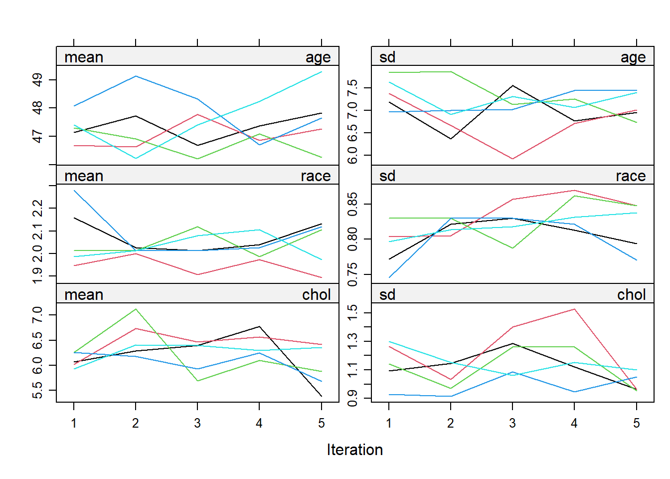
The line in the plot should be intermingled and free of any trend. The number of iteration can be further increased to make sure of this.
miImp2 <- mice.mids(miImp, maxit = 35, printFlag = F)
plot(miImp2)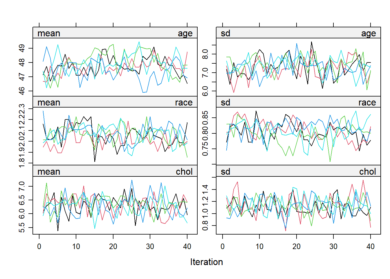
Once the imputed datasets are obtained, an analysis (for example, a linear regression) can be run as follows:
lr_mi <- with(miImp, glm(dbp ~ age + race + chol + cad + sbp + bmi + gender))
pool(lr_mi) %>%
  summary(conf.int = T)
## term estimate std.error statistic df p.value
## 1 (Intercept) 25.85805530 13.21741793 1.95636209 34.41840 0.05857610
## 2 age -0.09649575 0.21229624 -0.45453348 10.34947 0.65882968
## 3 raceindian -0.07034050 2.57995900 -0.02726419 12.32421 0.97868554
## 4 racemalay 0.20029789 1.68514315 0.11886105 59.44295 0.90578621
## 5 chol 1.33244955 0.52966992 2.51562245 89.92925 0.01365737
## 6 cadno cad -1.43834422 1.43322822 -1.00356956 160.05725 0.31710092
## 7 sbp 0.51358079 0.03015353 17.03219634 186.95165 0.00000000
## 8 bmi -0.35959227 0.20258274 -1.77503907 136.19191 0.07812525
## 9 genderwoman 1.30467626 1.04972267 1.24287709 185.09416 0.21548528
## 2.5 % 97.5 %
## 1 -0.9909476 52.70705817
## 2 -0.5673651 0.37437357
## 3 -5.6752310 5.53454998
## 4 -3.1711401 3.57173588
## 5 0.2801565 2.38474258
## 6 -4.2688212 1.39213272
## 7 0.4540959 0.57306569
## 8 -0.7602069 0.04102233
## 9 -0.7662831 3.37563562We can use mutate_if() from dplyr package to round up the numbers to two decimal points.
pool(lr_mi) %>%
  summary(conf.int = T) %>%
  as.data.frame() %>%
  mutate_if(is.numeric, round, 2)
## term estimate std.error statistic df p.value 2.5 % 97.5 %
## 1 (Intercept) 25.86 13.22 1.96 34.42 0.06 -0.99 52.71
## 2 age -0.10 0.21 -0.45 10.35 0.66 -0.57 0.37
## 3 raceindian -0.07 2.58 -0.03 12.32 0.98 -5.68 5.53
## 4 racemalay 0.20 1.69 0.12 59.44 0.91 -3.17 3.57
## 5 chol 1.33 0.53 2.52 89.93 0.01 0.28 2.38
## 6 cadno cad -1.44 1.43 -1.00 160.06 0.32 -4.27 1.39
## 7 sbp 0.51 0.03 17.03 186.95 0.00 0.45 0.57
## 8 bmi -0.36 0.20 -1.78 136.19 0.08 -0.76 0.04
## 9 genderwoman 1.30 1.05 1.24 185.09 0.22 -0.77 3.38mice package has provided an easy flow to run the analysis for multiple imputation:
mice(): impute the missing datawith(): run a statistical analysispool(): pool the results
Additionally, a model comparison can be done as well. There are three methods available for the model comparison:
D1(): multivariate Wald testD2(): pools test statistics from each analysis of the imputed datasetsD3(): likelihood-ratio test statistics
D2() is less powerful compared to the other two methods.
lr_mi2 <- with(miImp, glm(dbp ~ race + chol + cad + sbp + bmi + gender))
summary(D1(lr_mi, lr_mi2))
##
## Models:
## model formula
## 1 dbp ~ age + race + chol + cad + sbp + bmi + gender
## 2 dbp ~ race + chol + cad + sbp + bmi + gender
##
## Comparisons:
## test statistic df1 df2 dfcom p.value riv
## 1 ~~ 2 0.2066007 1 4 191 0.6730188 1.379672
##
## Number of imputations: 5 Method D1Multivariate Wald test is not significant. Hence, removing age from the model does not reduce its predictive power. We can safely exclude age variable to aim for a parsimonious model.
summary(D2(lr_mi, lr_mi2))##
## Models:
## model formula
## 1 dbp ~ age + race + chol + cad + sbp + bmi + gender
## 2 dbp ~ race + chol + cad + sbp + bmi + gender
##
## Comparisons:
## test statistic df1 df2 dfcom p.value riv
## 1 ~~ 2 -0.002254427 1 16.1953 NA 1 0.9879772
##
## Number of imputations: 5 Method D2 (wald)summary(D3(lr_mi, lr_mi2))##
## Models:
## model formula
## 1 dbp ~ age + race + chol + cad + sbp + bmi + gender
## 2 dbp ~ race + chol + cad + sbp + bmi + gender
##
## Comparisons:
## test statistic df1 df2 dfcom p.value riv
## 1 ~~ 2 0.1946719 1 10.83101 191 0.6677344 1.549127
##
## Number of imputations: 5 Method D3Also, we get a similar result from the remaining two methods for the model comparison. However, this may not always be the case. Generally, D1() and D3() are preferred and equally good for a sample size more than 200. However, for a small sample size (n < 200), D1() is better. Besides, D2() should be used with cautious especially in large datasets with many missing values as it may produce a false positive estimate.
13.7 Presentation
gtsummary package can be used for all the analyses run on the approaches of handling missing data that we have covered in this chapter. Here is an example to get a nice table using tbl_regression() from a linear regression model run on the multiple imputation approach.
tbl_regression(lr_mi2)| Characteristic | Beta | 95% CI | p-value |
|---|---|---|---|
| race | |||
| chinese | — | — | |
| indian | -0.86 | -4.1, 2.3 | 0.6 |
| malay | 0.73 | -2.0, 3.5 | 0.6 |
| chol | 1.3 | 0.29, 2.3 | 0.012 |
| cad | |||
| cad | — | — | |
| no cad | -1.3 | -4.0, 1.5 | 0.4 |
| sbp | 0.51 | 0.45, 0.57 | <0.001 |
| bmi | -0.36 | -0.77, 0.04 | 0.076 |
| gender | |||
| man | — | — | |
| woman | 1.4 | -0.67, 3.4 | 0.2 |
13.8 Resources
We suggest Schafer and Graham (2002) and Kang (2013) for theoretical details on the missing data, Zhang (2015) for missing data exploration and Martin W Heymans (2019) and Buuren (2018) for more details on single and multiple imputation.
13.9 Summary
This chapter provides an overview of the type of missing data and how to investigate it, either visually, descriptively or statistically. This chapter also covers practical methods for handling missing data in research from a simple method like a listwise deletion to a more advanced method of multiple imputation. There is extensive literature on the approach to missing data that are not included in this brief chapter. However, we hope this chapter will give readers a solid starting point to further explore other resources.