Chapter 12 Parametric Survival Analysis
12.1 Objectives
At the end of the chapter, readers will be able
- to understand the basic concept of parametric survival analysis
- to understand the common parametric survival analysis models such as the exponential regression model and the Weibull survival mode.
- to perform the analysis for the exponential regression model and the Weibull regression model
12.2 Introduction
In survival analysis, the Cox proportional hazard (PH) regression is very popular to model the association between the time-to-event with covariates or independent variables. It is also a form of Generalized Linear Models.Cox PH regression is a semi-parametric survival analysis model.
The Cox Proportional Hazard model is the most popular technique to analysis the effects of covariates on survival time but under certain circumstances parametric models may offer advantages over Cox’s model. In addition to Cox proportional hazard regression model, there is an additional class of survival models, called the parametric survival models. With parametric models such as linear regression, logistic regression and Poisson regression, the outcome is assumed to follow some distribution.
Researchers in medical sciences often tend to prefer semi-parametric instead of parametric models because of fewer assumptions but some comments recommended that under certain circumstances, parametric models estimate the parameter more efficient. In parametric models we often use maximum likelihood procedures to estimate the unknown parameters and this technique and its interpretation are familiar for researchers. Also accelerated failure time can be used as relative risk with similar interpretation in Cox PH regression.
In the parametric survival models, the distribution of the outcome (i.e. the time to event) is specified in terms if unknown parameters.The interests in parametric models include:
- determining the acceleration factor and/or
- determining the hazard ratio.
The common parametric models include:
- Exponential survival model
- Weibull survival model and
- log-logistic survival model.
12.2.1 Advantages of parametric survival analysis models
A fully parametric model has some advantages (Lemeshow, May, and Hosmer Jr. 2008):
- full maximum likelihood may be used to estimate the parameters
- the estimated coefficients or transformations of them can provide clinically meaningful estimates of effect
- fitted values from the model can provide estimates of survival time
- residuals can be computed as differences between observed and predicted values of time
An analysis of censored time-to-event data using a fully parametric model can almost have the look and feel of a normal-errors linear regression analysis.
12.3 Parametric survival analysis model
The shape of the survival or hazard curve is informative of the process and provides a link to substantive issues. Parametric models mean the outcome is assumed to follow some distributions. This also means that the outcome follows some family of distributions of similar form BUT with unknown parameters. In parametric survival analysis all parts of the model are specified, both the hazard function and the effect of any covariates.
The strength of this is that estimation is easier and estimated survival curves are smoother as they draw information from the whole data. The main drawback to parametric methods is that they require extra assumptions that may not be appropriate. Parametric models have proportional hazard metrics and accelerated failure time (AFT ) metrics. AFT models allow covariates to predict survival. Often, no analytic solution for the MLE exists. In such cases, a numerical approach must be taken. A popular method is to use Newton Raphson.
Again, a parametric survival model is one of which survival time (the outcome) is assumed to follow a known distribution. The parametric models specify the baseline hazard and the baseline hazard indicates which model to be used, for examples:
- Weibull model
- Log-logistic model
- Log-normal model
- Exponential model
- Generalized Gamma model
For parametric survival models, time is assumed to follow some distribution whose probability density function \(f(t)\) can be expressed in terms of unknown parameters. Once a probability density function is specified for survival time, the corresponding survival and hazard functions can be determined.
The survival function can be also expressed in terms of hazard function by exponentiating the negative cumulative hazard function.Probability density function can also be expressed as the product of the hazard and the survival function, \(f(t) =h(t)S(t)\)
Many parametric models are Accelerated Failure Time (AFT) models rather than Proportional Hazard models. And remember, Constant Hazard fulfills Proportional Hazard assumption but Proportional Hazard does not mean a model has Constant Hazard.
12.3.1 Proportional hazard parametric models
Parametric models can be presented either as a proportional hazard models or accelerated failure time (AFT) models. Parametric models that have both the proportional hazards models and accelerated failure time models are:
- Exponential model
- Weibull model
If we take the Exponential model as an example, in the exponential survival model with a single covariate, \(X\) then the hazard function for the proportional hazard model is:
\[h(t) = \exp^{(\beta_0 + \beta_1 x)}\] \[h(t) = \exp^{\beta_0} \exp^{\beta_1x}\] \[h(t) = h_0 \exp^{\beta_1x}\]
12.3.2 Accelerated failure time model (AFT) models
Again, if we take the Exponential model with a single covariate, \(X\) then the hazard function for the AFT model is
\[h(t) = \frac{1}{(\exp^{\alpha_0 + \alpha_1x})}\] \[h(t) = \exp^{\alpha_0}\exp^{\alpha_1x}\] \[h(t) = h_0 \exp^{-\alpha_1x}\]
A convenient and plausible way to characterize the distribution of time to event, denoted T, as a function of a single covariate is via the equation:
\[T = \exp^{\beta_0 + \beta_1x} \times \epsilon\]
For the exponential model, these are equivalent, but this is not true in general. In other parametric models, it is possible for a model to be proportional hazard models but not AFT, or AFT but not proportional hazard models, or both, or neither.
Because time must be positive, then:
- the systematic component, \(\exp^{\beta_0 + \beta_1x}\) must be positive
- the error component \(\epsilon\) must also be positive
We can linearize the model, by taking the natural log of each side of the equation. And, now it becomes:
\[ln(T) = \beta_0 + \beta_1x + \epsilon^*\]
The error component, \(\epsilon^*\) can follow different distribution. If the error component follows the exponential distribution then we call the model as the exponential regression model. Other possible distribution includes Weibull regression model, log-normal model, log-logistics and others.
Survival time models that can be linearized by taking logs are called accelerated failure time models. The effect of covariate is multiplicative (proportional) with respect to survival time. Whereas, for the PH models, the assumption is that; the effect of covariates is multiplicative with respect to hazard.
12.4 Analysis
This study was conducted from latest release data from the 2017 submission of the SEER database (1973 to 2015 data) of the National Cancer Institute. Patients with a diagnosis of AO were selected from the SEER database using the International Classification of Diseases for Oncology, Third Edition (ICD-O-3) histology code 9451. There are 1824 patients were diagnosed with AO in this dataset.
12.4.1 Dataset
The dataset contains all variables of our interest. For the purpose of this assignment, we want to explore prognostic factor association of age, surgery status and marital status with the survival of AO patients. The variables in the dataset as follow:
- age : biological age at the beginning of the study. This data in numerical values.
- surgery : is the patient has undergone surgery. Coded as “Yes” and “No”
- marital : Marital status at diagnosis. Coded as “single”, “married”, or “separated/divorced/widowed”.
- survivaltime : survival time in month. This data is in numerical values.
- status : survival status coded as “1 = died” and “0 = censored”
12.4.2 Set the enviroment
We use these packages:
- here to specify the location of the working directory
- tidyverse for exploratory data analysis, data wrangling and plotting.
- gtsummary to provide nice statistical tables
- broom to provide clean and polish table from the estimates
- flexsurve to perform flexible parametric survival analysis models for time-to-event data, including the generalized gamma, the generalized F and the Royston-Parmar spline model, and extensible to user-defined distributions.
- SurvRefCensCov to transforms output based Weibull distribution to a more natural parameterization.
## here() starts at D:/Data_Analysis_CRC_multivar_data_analysis_codes## ── Attaching core tidyverse packages ──────────────────────── tidyverse 2.0.0 ──
## ✔ dplyr 1.1.4 ✔ readr 2.1.5
## ✔ forcats 1.0.0 ✔ stringr 1.5.1
## ✔ ggplot2 3.5.1 ✔ tibble 3.2.1
## ✔ lubridate 1.9.3 ✔ tidyr 1.3.1
## ✔ purrr 1.0.2## ── Conflicts ────────────────────────────────────────── tidyverse_conflicts() ──
## ✖ dplyr::filter() masks stats::filter()
## ✖ dplyr::lag() masks stats::lag()
## ℹ Use the conflicted package (<http://conflicted.r-lib.org/>) to force all conflicts to become errors## Loading required package: survival## Registered S3 method overwritten by 'SurvRegCensCov':
## method from
## print.src dplyr12.4.3 Read dataset
## Rows: 1824 Columns: 8
## ── Column specification ────────────────────────────────────────────────────────
## Delimiter: ","
## chr (5): marital, sex, surgery, race, first
## dbl (3): age, status, survivaltime
##
## ℹ Use `spec()` to retrieve the full column specification for this data.
## ℹ Specify the column types or set `show_col_types = FALSE` to quiet this message.
12.4.4 Data Wrangling
We will select only these variables to simplify our model building process:
- age
- surgery
- marital
- survivaltime
- status
And then we will convert all character variables to factor variables.
d1<- d1 %>%
  dplyr::select(age, surgery, marital, survivaltime, status) %>%
  mutate_if(is.character, as.factor)
glimpse(d1)
## Rows: 1,824
## Columns: 5
## $ age <dbl> 4, 4, 4, 5, 5, 5, 6, 6, 6, 8, 9, 11, 11, 11, 11, 12, 13, …
## $ surgery <fct> Yes, Yes, Yes, Yes, No, No, Yes, Yes, Yes, Yes, Yes, Yes,…
## $ marital <fct> Single, Single, Single, Single, Single, Single, Single, S…
## $ survivaltime <dbl> 290, 9, 10, 141, 12, 54, 161, 60, 11, 8, 15, 298, 83, 15,…
## $ status <dbl> 0, 1, 1, 0, 1, 1, 0, 0, 1, 1, 1, 0, 0, 1, 1, 0, 1, 0, 1, …12.4.5 Exploratory Data Analysis (eda)
We will do simple eda
d1 %>%
  mutate(status = dplyr::recode(status,"0" = "Censored", "1" = "Death")) %>%
  tbl_summary(by = status,
              statistic = list(all_continuous() ~ "{mean} ({sd})",
                              all_categorical() ~ "{n} ({p}%)"),
              type = list(where(is.logical) ~ "categorical"),
              label = list(age ~ "Age (in years old)",
                           surgery ~ "Surgery Status",
                           marital~"Marital Status", survivaltime ~ "Time (month)"),
            missing_text = "Missing") %>%
  modify_caption("**Table 1. Patient Characteristic**")  %>%
  modify_header(label ~ "**Variable**") %>%
  modify_spanning_header(c("stat_1", "stat_2") ~ "**Survival Status**") %>%
  modify_footnote(all_stat_cols() ~ "Mean (SD) or Frequency (%)") %>%
  bold_labels() %>%
as_gt()| Variable | Survival Status | |
|---|---|---|
| Censored N = 8351 |
Death N = 9891 |
|
| Age (in years old) | 45 (13) | 52 (16) |
| Surgery Status | 774 (93%) | 835 (84%) |
| Marital Status | ||
| Married | 531 (64%) | 606 (61%) |
| Separated/divorced/widowed | 96 (11%) | 174 (18%) |
| Single | 208 (25%) | 209 (21%) |
| Time (month) | 83 (65) | 38 (42) |
| 1 Mean (SD) or Frequency (%) | ||
12.4.6 Exponential survival model
We can use the survreg() from survival package. However survreg() only perform estimation for AFT metric.
exp.mod.aft <- survreg(Surv(survivaltime, status) ~ age + marital + surgery,
                           data = d1, dist = 'exponential')
summary(exp.mod.aft)
##
## Call:
## survreg(formula = Surv(survivaltime, status) ~ age + marital +
## surgery, data = d1, dist = "exponential")
## Value Std. Error z p
## (Intercept) 6.6348 0.1601 41.45 < 2e-16
## age -0.0487 0.0025 -19.50 < 2e-16
## maritalSeparated/divorced/widowed -0.0609 0.0871 -0.70 0.48458
## maritalSingle -0.3068 0.0823 -3.73 0.00019
## surgeryYes 0.5250 0.0879 5.97 2.4e-09
##
## Scale fixed at 1
##
## Exponential distribution
## Loglik(model)= -5401.2 Loglik(intercept only)= -5614.4
## Chisq= 426.47 on 4 degrees of freedom, p= 5.3e-91
## Number of Newton-Raphson Iterations: 5
## n= 182412.4.7 Weibull (Accelerated Failure Time)
We first start with estimating a Weibull parametric survival model which will return a accelerated failure metric:
To do this, we will be using the survreg() function
wei.mod.aft <- survreg(Surv(survivaltime, status) ~ age + surgery + marital,
                        data = d1, dist = 'weibull')
summary(wei.mod.aft)
##
## Call:
## survreg(formula = Surv(survivaltime, status) ~ age + surgery +
## marital, data = d1, dist = "weibull")
## Value Std. Error z p
## (Intercept) 6.82050 0.19724 34.58 < 2e-16
## age -0.05270 0.00305 -17.26 < 2e-16
## surgeryYes 0.62515 0.10897 5.74 9.7e-09
## maritalSeparated/divorced/widowed -0.10037 0.10713 -0.94 0.3488
## maritalSingle -0.35437 0.10184 -3.48 0.0005
## Log(scale) 0.20727 0.02577 8.04 8.8e-16
##
## Scale= 1.23
##
## Weibull distribution
## Loglik(model)= -5365.4 Loglik(intercept only)= -5533.9
## Chisq= 336.93 on 4 degrees of freedom, p= 1.2e-71
## Number of Newton-Raphson Iterations: 5
## n= 1824However, the parameters estimated from survreg() does not make clinical sense. So, we will convert to log hazard ratio, hazard ratio and estimated time ratio. To do this, we will use the ConvertWeibull() to convert the Weibull PH to Weibul AFT model
## $vars
##                                       Estimate           SE
## lambda                             0.003912012 0.0007814675
## gamma                              0.812800295 0.0209455354
## age                                0.042835914 0.0025361397
## surgeryYes                        -0.508122220 0.0879913395
## maritalSeparated/divorced/widowed  0.081578034 0.0869994355
## maritalSingle                      0.288029086 0.0826554798
##
## $HR
##                                          HR        LB        UB
## age                               1.0437666 1.0385912 1.0489678
## surgeryYes                        0.6016242 0.5063222 0.7148644
## maritalSeparated/divorced/widowed 1.0849979 0.9149025 1.2867167
## maritalSingle                     1.3337961 1.1343132 1.5683606
##
## $ETR
##                                         ETR        LB        UB
## age                               0.9486630 0.9430040 0.9543559
## surgeryYes                        1.8685265 1.5091765 2.3134412
## maritalSeparated/divorced/widowed 0.9045057 0.7331977 1.1158390
## maritalSingle                     0.7016179 0.5746698 0.8566096
Or we can simply use flexsurv() to obtain the the log time ratio and time ratio.
wei.mod.aft <- flexsurvreg(Surv(survivaltime, status) ~ age + surgery + marital,
                           data = d1, dist = 'weibull')
wei.mod.aft
## Call:
## flexsurvreg(formula = Surv(survivaltime, status) ~ age + surgery +
## marital, data = d1, dist = "weibull")
##
## Estimates:
## data mean est L95% U95%
## shape NA 8.13e-01 7.73e-01 8.55e-01
## scale NA 9.16e+02 6.23e+02 1.35e+03
## age 4.89e+01 -5.27e-02 -5.87e-02 -4.67e-02
## surgeryYes 8.82e-01 6.25e-01 4.12e-01 8.39e-01
## maritalSeparated/divorced/widowed 1.48e-01 -1.00e-01 -3.10e-01 1.10e-01
## maritalSingle 2.29e-01 -3.54e-01 -5.54e-01 -1.55e-01
## se exp(est) L95% U95%
## shape 2.09e-02 NA NA NA
## scale 1.81e+02 NA NA NA
## age 3.05e-03 9.49e-01 9.43e-01 9.54e-01
## surgeryYes 1.09e-01 1.87e+00 1.51e+00 2.31e+00
## maritalSeparated/divorced/widowed 1.07e-01 9.05e-01 7.33e-01 1.12e+00
## maritalSingle 1.02e-01 7.02e-01 5.75e-01 8.57e-01
##
## N = 1824, Events: 989, Censored: 835
## Total time at risk: 106252
## Log-likelihood = -5365.418, df = 6
## AIC = 10742.8412.4.7.1 Interpretation for accelerated failure time
The interpretation of the parameters are as below:
The estimated log time ratio to die for every increment of 1 year of age was \(-0.0527\). The Acceleration Factor (AF) or Time Ratio (TR) is \(\exp(-0.0527)\) which equals \(0.949\). It means that for every 1 year increase of age, OA patients will die earlier (a factor of \(0.949\)). Or, we can say for every 1 year increase of age, the survival time for OA patients will be significantly shorter by \(5.1\%\) when adjusted for surgery status and marital status. The reduction in survival in OA patients could range between \(4.6\%\) and \(5.7\%\) (Adj. TR = \(0.949\), \(95\%\) CI = \(0.943,0.954\)).
The estimated log time ratio to die in OA patients who underwent surgery (in comparison to those who did not) was \(0.625\). The Acceleration Factor (AF) or Time Ratio (TR) is \(\exp(0.625)\) which equals \(1.87\). The survival time for OA patients who underwent surgery was estimated to be \(1.87\%\) times longer than of that of patients who did not undergo surgery. Or, it also means, the survival time among OA patients who underwent surgery was \(87.0\%\) longer than those who did not go for surgery, when adjusted for age and marital status. The increase duration of survival ranges between \(51.0\%\) and \(131.0\%\) (Adj. TR = 1.87, \(95\%\) CI = 1.51,2.31)
The estimated log time ratio to die in subjects who were single (in comparison to those who were married) was \(-0.354\). The Acceleration Factor (AF) or Time Ratio (TR) is \(\exp(-0.354)\) which equals \(0.702\). The survival time for OA patients who were single is shorter, estimated to be about a factor of \(70.2\%\) than OA patients who were married. The survival time among OA patients who were single was shorter by \(29.8\%\) when adjusted for surgery status and age. The survival shortened between \(14.3\%\) and \(42.5\%\) (Adj. TR = 0.702, \(95\%\) CI = 0.575,0.857).
The estimated log time ratio to die in subjects who were separated or divorced or widowed (in comparison to those are married) was \(-0.100\). The Acceleration Factor (AF) or Time Ratio (TR) is \(\exp(-0.100)\) which equals \(0.905\). This shows that the survival of OA patients who were separated or divorced or widowed was \(90.5\%\) as compared to OA patients who were married. The survival time in OA patients who were separated or divorced or widowed was shorter by \(9.5\%\) when adjusted for surgery status and age. The reduction is survival time ranged between \(26.7\%\) and \(12.0\%\) (Adj. TR = 0.905, \(95\%\) CI = 0.733,1.12).
12.4.8 Weibull (Proportional Hazard)
In contrast to AFT metric, the flexsurvreg() could convert the estimation to proportional hazard (PH) metric. Below, we will obtain the estimate for log hazard ratio and the hazard ratio with their \(95\%\) confidence intervals.
wei.mod.ph <- flexsurvreg(Surv(survivaltime, status) ~ age + surgery + marital,
                           data = d1, dist = 'weibullPH')
wei.mod.ph
## Call:
## flexsurvreg(formula = Surv(survivaltime, status) ~ age + surgery +
## marital, data = d1, dist = "weibullPH")
##
## Estimates:
## data mean est L95% U95%
## shape NA 0.812800 0.772767 0.854907
## scale NA 0.003912 0.002645 0.005787
## age 48.937500 0.042836 0.037865 0.047807
## surgeryYes 0.882127 -0.508122 -0.680582 -0.335662
## maritalSeparated/divorced/widowed 0.148026 0.081578 -0.088938 0.252094
## maritalSingle 0.228618 0.288029 0.126027 0.450031
## se exp(est) L95% U95%
## shape 0.020946 NA NA NA
## scale 0.000781 NA NA NA
## age 0.002536 1.043767 1.038591 1.048968
## surgeryYes 0.087991 0.601624 0.506322 0.714864
## maritalSeparated/divorced/widowed 0.086999 1.084998 0.914903 1.286717
## maritalSingle 0.082655 1.333796 1.134313 1.568361
##
## N = 1824, Events: 989, Censored: 835
## Total time at risk: 106252
## Log-likelihood = -5365.418, df = 6
## AIC = 10742.8412.4.8.1 Interpretation for proportional hazard metric
The log g hazard ratio for death among OA patients who underwent surgery to those who did not go for surgery was \(-0.508\) which equals to hazard ratio of of \(0.60\). It means the the hazard for death was \(39.9\%\) lower in OA patients who went for surgery as compared to OA patients who did not undergo surgery, adjusted for age and marital status. The reduction in risk for death ranges between \(29\%\) and \(50\%\) (Adj. HR = 0.601, \(95\%\) CI = 0.50,0.71).
An increase of 1 year of age would increase the log hazard by 0.043 or the risk (hazard) for death by \(4.4\%\) when adjusted for marital status and surgery status. The risk for death could increase between \(3.9\%\) and \(4.9\%\) (Adj. HR = 1.043, \(95\%\) CI = 1.039, 1.049).
OA Patients who were separated or widowed or divorced had higher risk (hazard) for death by \(8.5\%\) as compared to OA patients who were married, when adjusted for age and surgery status. The risk for death could be lower by \(9\%\) or higher by \(29\%\) (Adj. HR = 1.085, \(95\%\) CI = 0.91, 1.29).
OA patients who were single had an increase risk for death (by \(33\%\)) as compared to OA patients who were married, when adjusted for age and surgery status. The increase in the risk for death for single OA patients range between \(13\%\) and \(57\%\) (Adj. HR = 1.33, \(95\%\) CI = 1.13, 1.568).
12.4.9 Model adequacy for Weibull distribution
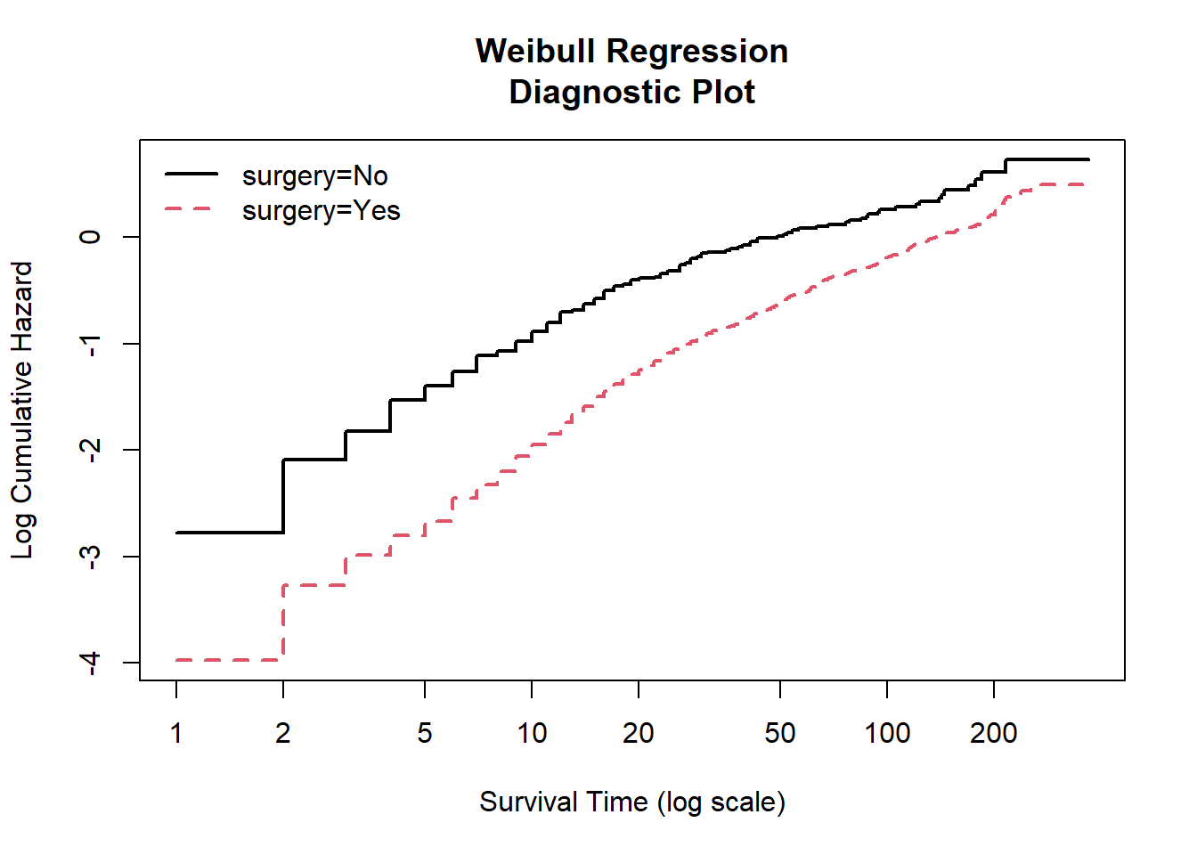
From the Weibull regression diagnostic plot, we can see that the lines for surgery status (yes and no) are generally parallel and linear in its scale. Thus, we can assume that the Weibull model is fit.
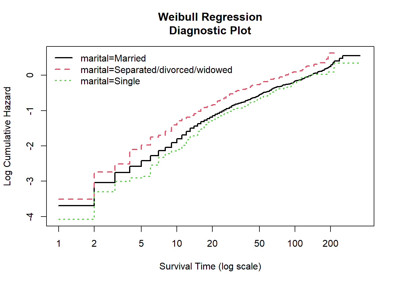
The Weibull regression diagnostic plot for marital status also shows rather parallel and linear lines. Again, we can assume that the Weibull model is fit.
12.5 Summary
In this chapter we learned briefly the concept of parametric survival analysis. We are also shown how to perform parametric survival analysis for the exponential regression model and the Weibull regression model. In each models, we further illustrate the accelerated failure time (AFT) and proportional hazed (PH) metrics. For more understanding, we recommend Survival Analysis: A Self-Learning Text book (D. G. Kleinbaum and Klein 2005) and Applied Survival Analysis: Regression Modeling of Time-to-Event Data book (Lemeshow, May, and Hosmer Jr. 2008).