Chapter 8 Binary Logistic Regression
8.1 Objectives
At the end of the chapter, the readers will be able
- to understand the concept of simple and multiple binary logistic regression
- to perform simple binary logistic regression
- to perform multiple binary logistic regression
- to perform model assessment of binary logistic regression
- to present and interpret results from binary logistic regression
8.2 Introduction
A binary variable is a categorical outcome that has two categories or levels. In medical and health research, the binary outcome variable is very common. Some examples where the outcome is binary include:
- survival status when the status of cancer patients at the end of treatment are coded as either alive or dead
- relapse status when the status of a patient is coded as either relapse or not relapse
- satisfaction level when patients who come to clinics are asked if they are satisfied or not satisfied with the service
- glucose control when patients were categorized as either good control or poor control based on Hba1c
In statistics, the logistic model (or logit model) is a statistical model that models the probability of an event taking place by having the log-odds for the event be a linear combination of one or more independent variables. In a binary logistic regression model, the dependent variable has two levels (categorical).
8.3 Logistic regression model
The logistic model (or logit model) is used to model the probability of a particular class or event existing, such as pass or fail, win or lose, alive or dead or healthy or sick.
More specifically, binary logistic regression is used to model the relationship between a covariate or a set of covariates and an outcome variable which is a binary variable.
8.4 Dataset
We will use a dataset named stroke.dta which in STATA format. These data come from a study of hospitalized stroke patients. The original dataset contains 12 variables, but our main variables of interest are:
- status : Status of patient during hospitalization (alive or dead)
- gcs : Glasgow Coma Scale on admission (range from 3 to 15)
- stroke_type : IS (Ischaemic Stroke) or HS (Haemorrhagic Stroke)
- sex : female or male
- dm : History of Diabetes (yes or no)
- sbp : Systolic Blood Pressure (mmHg)
- age : age of patient on admission
The outcome variable is variable status. It is labelled as either dead or alive, which is the outcome of each patient during hospitalization.
8.5 Logit and logistic models
The simple binary logit and logistic models refer to a a model with only one covariate (also known as independent variable). For example, if the covariate is gcs (Glasgow Coma Scale), the simple logit model is written as:
\[\hat{g}(x)= ln\left[ \frac{\hat\pi(x)}{1 - {\hat\pi(x)}} \right]\]
where \(\hat{g}(x)\) is the log odds for death for a given value of gcs. And the odds for death for a given value of GCS is written as \(= \hat\beta_0 + \hat\beta_1(gcs)\)
And the simple logistic model is also written as:
\[\hat{\pi}(x) = \frac{exp^{\hat{\beta}_{0} + \hat{\beta}_{1}{gcs}}}{1 + exp^{\hat{\beta}_{0} + \hat{\beta}_{1}{gcs}}}\] The \(\pi(x) = E(Y|x)\) represents the conditional mean of \(Y\) given \(x\) when the logistic distribution is used. This is also simply known as the predicted probability of death for given value of gcs.
If we have decided (based on our clinical expertise and literature review) that a model that could explain death consists of gcs, stroke type, sex, dm, age and sbp, then the logit model can be expanded to:
\[\hat{g}(x) = \hat\beta_0 + \hat\beta_1(gcs) + \hat\beta_2(stroke type) + \hat\beta_3(sex)+ \hat\beta_4(dm) + \hat\beta_5(sbp) + \hat\beta_6(age)\]
These are the odds for death given certain gcs, sbp and age values and specific categories of stroke type, sex and diabetes. While the probability of death is
\[\hat{\pi}(x) = \frac{exp^{\hat\beta_0 + \hat\beta_1(gcs) + \hat\beta_2(stroke type) + \hat\beta_3(sex)+ \hat\beta_4(dm) + \hat\beta_5(sbp) + \hat\beta_6(age)})}{1 + exp^{\hat\beta_0 + \hat\beta_1(gcs) + \hat\beta_2(stroke type) + \hat\beta_3(sex)+ \hat\beta_4(dm) + \hat\beta_5(sbp) + \hat\beta_6(age)}}\]
In many datasets, some independent variables are either discrete or nominal scale variables. Such variables include race, sex, treatment group, and age categories. Including them in the model is inappropriate as if they were interval scale variables is inappropriate. In some statistical software, these variables are represented by numbers. However, be careful; these numbers are used merely as identifiers or labels for the groups.
In this situation, we will use a method called design variables (or dummy variables). Suppose, for example, assuming that one of the independent variables is obesity type, which is now coded as “Class 1”, “Class 2” and “Class 3”. In this case, there are 3 levels or categories, hence two design variables (\(D - 1\)) are necessary, let’s say D1 and D2. One possible coding strategy is that when the patient is in “Class 1” then the two design variables, for D1 and D2 would both be set equal to zero. In this example, “Class 1” is the reference category. When the patient is in “Class 2”, then D1 is set as 1 and D2 as 0; when the patient is in “Class 3”, the we will set D1 as 0 and D2 and 1. All these coding assignments can be done automatically in the software. But to interpret, we must know which category is the reference.
8.6 Prepare environment for analysis
8.6.1 Creating a RStudio project
Start a new analysis task by creating a new RStudio project. To do this,
- Go to File
- Click New Project
- Choose New Directory or Existing Directory.
This directory points to the folder that usually contains the dataset to be analyzed. This is called as the working directory. Make sure there is a folder named as data in the folder. If there is not, create one. Make sure the dataset stroke.dta is inside the data folder in the working directory.
8.6.2 Loading libraries
Next, we will load the necessary packages. We will use 5 packages
- the built in stat package - to run Generalized Linear Model. This is already loaded by default.
- haven - to read SPSS, STATA and SAS dataset
- tidyverse - to perform data transformation
- gtsummary - to provide nice results in a table
- broom - to tidy up the results
- LogisticDx - to do model assessment
- here - to ensure proper directory
To load these packages, we will use the function library():
## ── Attaching core tidyverse packages ──────────────────────── tidyverse 2.0.0 ──
## ✔ dplyr     1.1.4     ✔ readr     2.1.5
## ✔ forcats   1.0.0     ✔ stringr   1.5.1
## ✔ ggplot2   3.5.1     ✔ tibble    3.2.1
## ✔ lubridate 1.9.3     ✔ tidyr     1.3.1
## ✔ purrr     1.0.2
## ── Conflicts ────────────────────────────────────────── tidyverse_conflicts() ──
## ✖ dplyr::filter() masks stats::filter()
## ✖ dplyr::lag()    masks stats::lag()
## ℹ Use the conflicted package (<http://conflicted.r-lib.org/>) to force all conflicts to become errors## here() starts at D:/Data_Analysis_CRC_multivar_data_analysis_codes8.7 Read data
WE will read data in the working directory into our R environment. The example dataset comes from a study among stroke inpatients. The dataset is in the STATA format stroke.dta.
Take a peek at data to check for
- variable names
- variable types
## Rows: 226
## Columns: 7
## $ sex         <dbl+lbl> 1, 1, 1, 2, 1, 2, 2, 1, 2, 2, 1, 2, 2, 2, 2, 1, 2, 1, …
## $ status      <dbl+lbl> 1, 1, 1, 1, 1, 1, 2, 1, 1, 2, 1, 1, 1, 1, 1, 1, 1, 1, …
## $ gcs         <dbl> 13, 15, 15, 15, 15, 15, 13, 15, 15, 10, 15, 15, 15, 15, 15…
## $ sbp         <dbl> 143, 150, 152, 215, 162, 169, 178, 180, 186, 185, 122, 211…
## $ dm          <dbl+lbl> 0, 0, 0, 1, 1, 1, 1, 0, 1, 1, 0, 1, 1, 1, 0, 1, 1, 1, …
## $ age         <dbl> 50, 58, 64, 50, 65, 78, 66, 72, 61, 64, 63, 59, 64, 62, 40…
## $ stroke_type <dbl+lbl> 0, 0, 0, 0, 0, 0, 0, 0, 0, 0, 0, 0, 0, 0, 0, 0, 0, 0, …
8.8 Explore data
Variables sex, status, dm and stroke type are labelled variables though they are coded as numbers. The numbers represent the groups or categories or levels of the variables. They are categorical variables and not real numbers.
We will transform all of labelled variables to factor variables using mutate(). And to transform all labelled variables, we can quickly achieve that by using the function across(). See the codes below to transform all labelled variables in the dataset to factor variables:
Now, examine the summary statistics:
| Characteristic | N = 2261 |
|---|---|
| sex | |
| male | 97 (43%) |
| female | 129 (57%) |
| alive or dead | |
| alive | 171 (76%) |
| dead | 55 (24%) |
| earliest Glasgow Coma Scale | 15.0 (10.0, 15.0) |
| earliest systolic BP (mmHg) | 161 (143, 187) |
| diabetes (yes or no) | 138 (61%) |
| age in years | 61 (52, 69) |
| Ischaemic Stroke or Haemorrhagic | |
| Ischaemic Stroke | 149 (66%) |
| Haemorrhagic | 77 (34%) |
| 1 n (%); Median (Q1, Q3) | |
If we want to get summary statistics based on the status of patients at discharge:
| Characteristic | alive N = 1711 |
dead N = 551 |
|---|---|---|
| sex | ||
| male | 81 (47%) | 16 (29%) |
| female | 90 (53%) | 39 (71%) |
| earliest Glasgow Coma Scale | 15.0 (14.0, 15.0) | 8.0 (5.0, 11.0) |
| earliest systolic BP (mmHg) | 160 (143, 186) | 162 (139, 200) |
| diabetes (yes or no) | 100 (58%) | 38 (69%) |
| age in years | 61 (53, 68) | 62 (50, 74) |
| Ischaemic Stroke or Haemorrhagic | ||
| Ischaemic Stroke | 132 (77%) | 17 (31%) |
| Haemorrhagic | 39 (23%) | 38 (69%) |
| 1 n (%); Median (Q1, Q3) | ||
8.9 Estimate the regression parameters
As we assume the outcome variable (status) follows binomial distribution, we will perform binary logistic regression. Logistic regression allow us to estimate the regression parameters \(\hat\beta_s\) or the log odds is dataset where the outcome follows binomial or bernoulli distribution.
To achieve the objective above, we do this in two steps:
- The simple binary logistic regression or the univariable logistic regression: In this analysis, there is only one independent variable or covariate in the model. This is also known as the crude or unadjusted analysis.
- The multiple binary logistic regression or the multivariable logistic regression: Here, we expand our model and include two or more independent variables (covariates). The multiple binary logistic regression model is an adjusted model, and we can obtain the estimate of a particular covariate independent of the other covariates in the model.
8.10 Simple binary logistic regression
Simple binary logistic regression model has a dependent variable and only one independent (covariate) variable.
In our dataset, for example, we are interested to model a simple binary logistic regression using
- status as the dependent variable.
- gcs as the independent variable.
The independent variable can be a numerical or a categorical variable.
To estimate the log odds (the regression parameters, \(\beta\)) for the covariate Glasgow Coma Scale (GCS), we can write the logit model as:
\[log\frac{p(status = dead)}{1 - p(status = dead)} = \hat\beta_0 + \hat\beta_1(gcs)\]
In R, we use the glm() function to estimate the regression parameters and other parameters of interest. Let’s run the model with gcs as the covariate and name the model as fatal_glm_1
To get the summarized result of the model fatal_glm_1, we will use the summary() function:
##
## Call:
## glm(formula = status ~ gcs, family = binomial(link = "logit"),
##     data = fatal)
##
## Coefficients:
##             Estimate Std. Error z value Pr(>|z|)
## (Intercept)  3.29479    0.60432   5.452 4.98e-08 ***
## gcs         -0.38811    0.05213  -7.446 9.64e-14 ***
## ---
## Signif. codes:  0 '***' 0.001 '**' 0.01 '*' 0.05 '.' 0.1 ' ' 1
##
## (Dispersion parameter for binomial family taken to be 1)
##
##     Null deviance: 250.83  on 225  degrees of freedom
## Residual deviance: 170.92  on 224  degrees of freedom
## AIC: 174.92
##
## Number of Fisher Scoring iterations: 5
To get the model summary in a data frame format, so we can edit more easily, we can use the tidy() function from the broom package. The package also contains other functions to provide other parameters useful for us later.
The function conf.int() will provide the confidence intervals (CI). The default is set at the \(95%\) level:
## # A tibble: 2 × 7
##   term        estimate std.error statistic  p.value conf.low conf.high
##   <chr>          <dbl>     <dbl>     <dbl>    <dbl>    <dbl>     <dbl>
## 1 (Intercept)    3.29     0.604       5.45 4.98e- 8    2.17      4.55
## 2 gcs           -0.388    0.0521     -7.45 9.64e-14   -0.497    -0.292
The estimates here are the log odds for death for a given value of gcs. In this example, each unit increase in gcs, the crude or unadjusted log odds for death due to stroke change by a factor \(-0.388\) with \(95%\) CI ranges from \(-0.497 and -0.292\).
Now, let’s use another covariate, stroke_type. Stroke type has 2 levels or categories; Haemorrhagic Stroke (HS) and Ischaemic Stroke (IS). HS is known to cause a higher risk for deaths in stroke. We will model stroke type (stroke_type), name the model as fatal_glm_2 and show the result using tidy()
fatal_glm_2 <-
  glm(status ~ stroke_type,
      data = fatal,
      family = binomial(link = 'logit'))
tidy(fatal_glm_2, conf.int = TRUE)
## # A tibble: 2 × 7
## term estimate std.error statistic p.value conf.low conf.high
## <chr> <dbl> <dbl> <dbl> <dbl> <dbl> <dbl>
## 1 (Intercept) -2.05 0.258 -7.95 1.80e-15 -2.59 -1.57
## 2 stroke_typeHaemorrha… 2.02 0.344 5.88 4.05e- 9 1.36 2.72The simple binary logistic regression models shows that patients with Haemorrhagic Stroke (HS) had a higher log odds for death during admission (by a factor \(2.02\)) as compared to patients with Ischaemic Stroke (IS).
8.11 Multiple binary logistic regression
There are multiple factors that can contribute to the outcome of stroke. Hence, there is a strong motivation to include other independent variables or covariates in the model. For example, in the case of stroke:
- It is unlikely that only one variable (gcs or stroke type) is related with stroke. Stroke like other cardiovascular diseases has many factors affecting the outcome. It makes more sense to consider adding other independent variables that we believe are important independent variables for stroke outcome in the model.
- by adding more covariates in the model, we can estimate the adjusted log odds. These log odds indicate the relationship of a particular covariate independent of other covariates in the model. In epidemiology, we always can this as adjustment. An adjustment is important particularly when we have confounding effects from other independent variables.
- interaction term can be generated (the product of two covariates) and added to the model to be estimated.
To add or not to add variables is a big subject on its own. Usually it is governed by clinical experience, subject matter experts and some preliminary analysis. You may read the last chapter of the book to understand more about model building and variable selection.
Let’s expand our model and include gcs, stroke type, sex, dm, sbp and age in the model. We will name this model as fatal_mv. As we have more than one independent variables in the model, we will call this as multiple binary logistic regression.
To estimates the multiple logistic regression model in R:
fatal_mv1 <-
  glm(status ~ gcs + stroke_type + sex + dm + sbp + age,
      data = fatal,
      family = binomial(link = 'logit'))
summary(fatal_mv1)
##
## Call:
## glm(formula = status ~ gcs + stroke_type + sex + dm + sbp + age,
## family = binomial(link = "logit"), data = fatal)
##
## Coefficients:
## Estimate Std. Error z value Pr(>|z|)
## (Intercept) -0.1588269 1.6174965 -0.098 0.92178
## gcs -0.3284640 0.0557574 -5.891 3.84e-09 ***
## stroke_typeHaemorrhagic 1.2662764 0.4365882 2.900 0.00373 **
## sexfemale 0.4302901 0.4362742 0.986 0.32399
## dmyes 0.4736670 0.4362309 1.086 0.27756
## sbp 0.0008612 0.0060619 0.142 0.88703
## age 0.0242321 0.0154010 1.573 0.11562
## ---
## Signif. codes: 0 '***' 0.001 '**' 0.01 '*' 0.05 '.' 0.1 ' ' 1
##
## (Dispersion parameter for binomial family taken to be 1)
##
## Null deviance: 250.83 on 225 degrees of freedom
## Residual deviance: 159.34 on 219 degrees of freedom
## AIC: 173.34
##
## Number of Fisher Scoring iterations: 5We could get a cleaner result in a data frame format (and you can edit in spreadsheet easily) of the multivariable model by using tidy() function:
## # A tibble: 7 × 7
##   term                   estimate std.error statistic p.value conf.low conf.high
##   <chr>                     <dbl>     <dbl>     <dbl>   <dbl>    <dbl>     <dbl>
## 1 (Intercept)            -1.59e-1   1.62      -0.0982 9.22e-1 -3.38       3.01
## 2 gcs                    -3.28e-1   0.0558    -5.89   3.84e-9 -0.444     -0.224
## 3 stroke_typeHaemorrhag…  1.27e+0   0.437      2.90   3.73e-3  0.411      2.13
## 4 sexfemale               4.30e-1   0.436      0.986  3.24e-1 -0.420      1.30
## 5 dmyes                   4.74e-1   0.436      1.09   2.78e-1 -0.368      1.35
## 6 sbp                     8.61e-4   0.00606    0.142  8.87e-1 -0.0110     0.0129
## 7 age                     2.42e-2   0.0154     1.57   1.16e-1 -0.00520    0.0555
We could see that the multivariable model that we named as fatal_mv1, can be interpreted as below:
- with one unit increase in Glasgow Coma Scale (GCS), the log odds for death during hospitalization equals to \(-0.328\), adjusting for other covariates.
- patients with HS have \(1.266\) times the log odds for death as compared to patients with IS, adjusting for other covariates.
- female patients have \(0.430\) times the log odds for death as compared to male patients, adjusting for other covariates.
- patients with diabetes mellitus have \(0.474\) times the log odds for deaths as compared to patients with no diabetes mellitus.
- With one mmHg increase in systolic blood pressure, the log odds for deaths change by a factor of \(0.00086\), when adjusting for other variables.
- with an increase in one year of age, the log odds for deaths change by a factor of \(0.024\), when adjusting for other variables.
In this book, we use the term independent variables, covariates and predictors interchangeably.
8.12 Convert the log odds to odds ratio
Lay person has difficulty to interpret log odds from logistic regression. That’s why, it is more common to interpret the logistic regression models using odds ratio. To obtain the odds ratios, we set the argument exponentiate = TRUE in the tidy() function. Actually, odds ratio can be easily calculate by \(\exp^{\beta_i}\)
## # A tibble: 7 × 7
##   term                   estimate std.error statistic p.value conf.low conf.high
##   <chr>                     <dbl>     <dbl>     <dbl>   <dbl>    <dbl>     <dbl>
## 1 (Intercept)               0.853   1.62      -0.0982 9.22e-1   0.0341    20.3
## 2 gcs                       0.720   0.0558    -5.89   3.84e-9   0.641      0.799
## 3 stroke_typeHaemorrhag…    3.55    0.437      2.90   3.73e-3   1.51       8.45
## 4 sexfemale                 1.54    0.436      0.986  3.24e-1   0.657      3.69
## 5 dmyes                     1.61    0.436      1.09   2.78e-1   0.692      3.87
## 6 sbp                       1.00    0.00606    0.142  8.87e-1   0.989      1.01
## 7 age                       1.02    0.0154     1.57   1.16e-1   0.995      1.06
8.13 Making inference
Let us rename the table appropriately so we can combine the results from the log odds and the odds ratio later.
## New names:
## • `term` -> `term...1`
## • `estimate` -> `estimate...2`
## • `std.error` -> `std.error...3`
## • `statistic` -> `statistic...4`
## • `p.value` -> `p.value...5`
## • `conf.low` -> `conf.low...6`
## • `conf.high` -> `conf.high...7`
## • `term` -> `term...8`
## • `estimate` -> `estimate...9`
## • `std.error` -> `std.error...10`
## • `statistic` -> `statistic...11`
## • `p.value` -> `p.value...12`
## • `conf.low` -> `conf.low...13`
## • `conf.high` -> `conf.high...14`
tab_logistic %>%
select(term...1, estimate...2, std.error...3,
estimate...9, conf.low...13, conf.high...14 ,p.value...5) %>%
rename(covariate = term...1,
log_odds = estimate...2,
SE = std.error...3,
odds_ratio = estimate...9,
lower_OR = conf.low...13,
upper_OR = conf.high...14,
p.val = p.value...5) ## # A tibble: 7 × 7
## covariate log_odds SE odds_ratio lower_OR upper_OR p.val
## <chr> <dbl> <dbl> <dbl> <dbl> <dbl> <dbl>
## 1 (Intercept) -0.159 1.62 0.853 0.0341 20.3 9.22e-1
## 2 gcs -0.328 0.0558 0.720 0.641 0.799 3.84e-9
## 3 stroke_typeHaemorrhagic 1.27 0.437 3.55 1.51 8.45 3.73e-3
## 4 sexfemale 0.430 0.436 1.54 0.657 3.69 3.24e-1
## 5 dmyes 0.474 0.436 1.61 0.692 3.87 2.78e-1
## 6 sbp 0.000861 0.00606 1.00 0.989 1.01 8.87e-1
## 7 age 0.0242 0.0154 1.02 0.995 1.06 1.16e-1In the model, we can interpret the estimates as below:
- if gcs increases by 1 unit (when stroke type is adjusted), the log odds for death changes by a factor \(-0.32\) or the odds for death changes by a factor \(0.72\) (odds for death reduces for \(28\%\)). The \(95\%CI\) are between \(21\%,36\%\), adjusting for other covariates.
- patients with HS have \(3.55\%\) times higher odds for stroke deaths - with \(95\%CI : 17\%, 85\%\) - as compared to patients with HS, adjusting for other independent variables.
- female patients have \(53\%\) higher odds for death as compared to female patients (\(p = 0.154\)), adjusting for other covariates.
- patients with diabetes mellitus have \(60.6\%\) higher odds for deaths compared to patients with no diabetes mellitus though the p value is above \(5\%\) (\(p = 0.642\%\)).
- With one mmHg increase in systolic blood pressure, the odds for death change by a factor \(1.00086\), when adjusting for other variables. The p value is also larger than \(5\%\).
- with an increase in one year of age, the odds for deaths increase by a factor of \(1.025\), when adjusting for other variables. However, the p value is \(0.115\)
8.14 Models comparison
The importance of independent variables in the models should not be based on their p-values or the Wald statistics alone. It is recommended to use likelihood ratio to compare models. The difference in the likelihood ratio between models can guide us on choosing a better model.
For example, when we compare model 1 (fatal_mv) and model 2 (fatal_glm_1), could we say that they are different? One approach is to to see if both models are different statistically. This comparison can be done by setting the level of significance at \(5\%\).
## Analysis of Deviance Table
##
## Model 1: status ~ gcs
## Model 2: status ~ gcs + stroke_type + sex + dm + sbp + age
##   Resid. Df Resid. Dev Df Deviance Pr(>Chi)
## 1       224     170.92
## 2       219     159.34  5   11.582  0.04098 *
## ---
## Signif. codes:  0 '***' 0.001 '**' 0.01 '*' 0.05 '.' 0.1 ' ' 1
Both models are different statistically (at \(5\%\) level). Hence, we prefer to keep model fatal_mv1 because the model makes more sense (more parsimonious).
Now, let’s be economical, and just keep variables such as gcs, stroke type and age in the model. We will name this multivariable logistic model as fatal_mv2:
And we will perform model comparison again:
## Analysis of Deviance Table
##
## Model 1: status ~ gcs + stroke_type + sex + dm + sbp + age
## Model 2: status ~ gcs + stroke_type + age
##   Resid. Df Resid. Dev Df Deviance Pr(>Chi)
## 1       219     159.34
## 2       222     161.51 -3  -2.1743    0.537
The p-value is above the threshold of \(5\%\) set by us. Hence, we do not want to reject the null hypothesis (null hypothesis says that both models are not statistically different). Our approach also agrees with Occam’s razor principle; always choose simpler model. In this case, fatal_mv2 is simpler and deserves further exploration.
8.15 Adding an interaction term
Interaction effect occurs when the effect of one variable depends on the value of another variable (in the case of two interacting variables). Interaction effect is common in regression analysis, ANOVA, and in designed experiments.
Two way interaction term involves two risk factors and their effect on one disease outcome. If the effect of one risk factor is the same within strata defined by the other, then there is no interaction. When the effect of one risk factor is different within strata defined by the other, then there is an interaction; this can be considered as a biological interaction.
Statistical interaction in the regression model can be measured based on the ways that risks are calculated (modeling). The presence of statistical interaction may not reflect true biological interaction.
Let’s add an interaction term between stroke type and diabetes:
fatal_mv2_ia <-
  glm(status ~ gcs + stroke_type + stroke_type:gcs + age,
      data = fatal,
      family = binomial(link = 'logit'))
tidy(fatal_mv2_ia)
## # A tibble: 5 × 5
## term estimate std.error statistic p.value
## <chr> <dbl> <dbl> <dbl> <dbl>
## 1 (Intercept) 0.508 1.37 0.371 0.710
## 2 gcs -0.320 0.0800 -4.01 0.0000619
## 3 stroke_typeHaemorrhagic 1.61 1.30 1.24 0.217
## 4 age 0.0236 0.0147 1.60 0.109
## 5 gcs:stroke_typeHaemorrhagic -0.0347 0.111 -0.312 0.755\[\hat{g}(x) = \hat\beta_0 + \hat\beta_1(gcs) + \hat\beta_2(stroke type) + \hat\beta_3(age)+ \hat\beta_4(gcs \times stroke_type)\]
To decide if we should keep an interaction term in the model, we should consider if the interaction term indicates both biological and statistical significance. If we believe that the interaction reflects both, then we should keep the interaction term in the model.
Using our data, we can see that:
- the coefficient for the interaction term for stroke type and gcs is not significant at the level of significance of \(5\%\) that we set.
- stroke experts also believe that the effect of gcs on stroke death is not largely different between different stroke type
Using both reasons, we decide not to keep the two-way interaction between gcs and stroke type in our multivariable logistic model.
8.16 Prediction from binary logistic regression
The broom package has a function called augment() which can calculate:
- estimated log odds
- probabilities
- residuals
- hat values
- Cooks distance
- standardized residuals
8.16.1 Predict the log odds
To obtain the .fitted column for the estimated log odds for death of each patient in the stroke data, we can run:
## # A tibble: 10 × 10
##    status   gcs stroke_type        age .fitted .resid    .hat .sigma   .cooksd
##    <fct>  <dbl> <fct>            <dbl>   <dbl>  <dbl>   <dbl>  <dbl>     <dbl>
##  1 alive     13 Ischaemic Stroke    50   -2.49 -0.398 0.00991  0.854 0.000209
##  2 alive     15 Ischaemic Stroke    58   -2.98 -0.314 0.00584  0.855 0.0000748
##  3 alive     15 Ischaemic Stroke    64   -2.84 -0.337 0.00590  0.855 0.0000871
##  4 alive     15 Ischaemic Stroke    50   -3.17 -0.287 0.00657  0.855 0.0000698
##  5 alive     15 Ischaemic Stroke    65   -2.82 -0.341 0.00599  0.855 0.0000904
##  6 alive     15 Ischaemic Stroke    78   -2.51 -0.395 0.00980  0.854 0.000203
##  7 dead      13 Ischaemic Stroke    66   -2.12  2.11  0.00831  0.843 0.0176
##  8 alive     15 Ischaemic Stroke    72   -2.65 -0.369 0.00731  0.855 0.000131
##  9 alive     15 Ischaemic Stroke    61   -2.91 -0.325 0.00579  0.855 0.0000796
## 10 dead      10 Ischaemic Stroke    64   -1.15  1.69  0.0173   0.847 0.0141
## # ℹ 1 more variable: .std.resid <dbl>
The slice() gives the snapshot of the data. In this case, we choose the first 10 patients.
8.16.2 Predict the probabilities
To obtain the .fitted column for the estimated probabilities for death of each patient, we specify type.predict = "response":
## # A tibble: 10 × 10
##    status   gcs stroke_type        age .fitted .resid    .hat .sigma   .cooksd
##    <fct>  <dbl> <fct>            <dbl>   <dbl>  <dbl>   <dbl>  <dbl>     <dbl>
##  1 alive     13 Ischaemic Stroke    50  0.0763 -0.398 0.00991  0.854 0.000209
##  2 alive     15 Ischaemic Stroke    58  0.0482 -0.314 0.00584  0.855 0.0000748
##  3 alive     15 Ischaemic Stroke    64  0.0551 -0.337 0.00590  0.855 0.0000871
##  4 alive     15 Ischaemic Stroke    50  0.0403 -0.287 0.00657  0.855 0.0000698
##  5 alive     15 Ischaemic Stroke    65  0.0564 -0.341 0.00599  0.855 0.0000904
##  6 alive     15 Ischaemic Stroke    78  0.0750 -0.395 0.00980  0.854 0.000203
##  7 dead      13 Ischaemic Stroke    66  0.107   2.11  0.00831  0.843 0.0176
##  8 alive     15 Ischaemic Stroke    72  0.0658 -0.369 0.00731  0.855 0.000131
##  9 alive     15 Ischaemic Stroke    61  0.0516 -0.325 0.00579  0.855 0.0000796
## 10 dead      10 Ischaemic Stroke    64  0.241   1.69  0.0173   0.847 0.0141
## # ℹ 1 more variable: .std.resid <dbl>
8.17 Model fitness
The basic logistic regression model assessment includes the measurement of overall model fitness. To do this, we check
- area under the curve
- Hosmer-Lemeshow test
- modidied Hosmer-Lemeshow test
- Oseo Rojek test
A fit model will not produce a large difference between the observed (from data) and the predicted values (from model). The difference is usually compared using p-values. If the p-values from the fit test show value of bigger than 0.05, then the test indicates that there is no significant difference between the observed data and the predicted values. Hence, will support that the model has good fit.
## Setting levels: control = 0, case = 1## Setting direction: controls < cases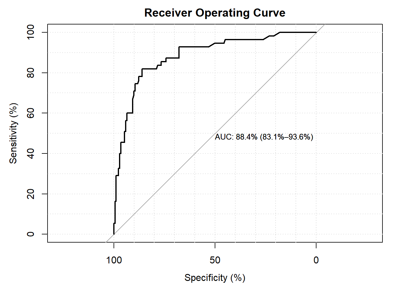
##          test   stat       val    df      pVal
##        <char> <char>     <num> <num>     <num>
## 1:         HL  chiSq  4.622183     6 0.5930997
## 2:        mHL      F  1.071882     7 0.3844230
## 3:       OsRo      Z -0.501724    NA 0.6158617
## 4: SstPgeq0.5      Z  1.348843    NA 0.1773873
## 5:   SstPl0.5      Z  1.516578    NA 0.1293733
## 6:    SstBoth  chiSq  4.119387     2 0.1274931
## 7: SllPgeq0.5  chiSq  1.579811     1 0.2087879
## 8:   SllPl0.5  chiSq  2.311910     1 0.1283862
## 9:    SllBoth  chiSq  2.341198     2 0.3101811
Our model shows that:
- the area under the curve is \(87.2\%\). The values of above 80 are considered to have good discriminating effect.
- the p-values from the Hosmer Lemeshow, the modified Hosmer Lemeshow and the Oseo Rojek are all above \(5\%\) values. This support our believe that our model has good fit.
8.18 Presentation of logistic regression model
The gtsummary package has a useful function tbld_regression() which can be used to produce a formatted table suitable for publication. For example, to generate a table for adjusted log odds ratio derived from our multivariable logistic regression model fatal_mv2, we can use the codes below:
| Characteristic | log(OR)1 | 95% CI1 | p-value |
|---|---|---|---|
| earliest Glasgow Coma Scale | -0.34 | -0.45, -0.24 | <0.001 |
| Ischaemic Stroke or Haemorrhagic | |||
| Ischaemic Stroke | — | — | |
| Haemorrhagic | 1.2 | 0.38, 2.1 | 0.004 |
| age in years | 0.02 | 0.00, 0.05 | 0.11 |
| 1 OR = Odds Ratio, CI = Confidence Interval | |||
Next, to generate the adjusted odds ratios table:
| Characteristic | OR1 | 95% CI1 | p-value |
|---|---|---|---|
| earliest Glasgow Coma Scale | 0.71 | 0.64, 0.79 | <0.001 |
| Ischaemic Stroke or Haemorrhagic | |||
| Ischaemic Stroke | — | — | |
| Haemorrhagic | 3.40 | 1.46, 7.97 | 0.004 |
| age in years | 1.02 | 1.00, 1.05 | 0.11 |
| 1 OR = Odds Ratio, CI = Confidence Interval | |||
8.19 Summary
In this chapter, we briefly explain that when readers want to model the relationship of a single or multiple independent variables with a binary outcome, then one of the analyses of choice is binary logit or logistic regression model. Then, we demonstrated simple and multiple binary logistic regression using glm() function and making predictions from the logistic regression model. Lastly, using gtsummary package readers can quickly create a nice regression table.
There are a number of good references to help readers understand binary logistic regression better. The references that we list below also contains workflow that will be useful for readers when modelling logistic regression. We highly recommend readers to read Applied Logistic Regression (Hosmer, Lemeshow, and Sturdivant 2013), Logistic Regression: Self Learning Text (D. Kleinbaum 2010) to strengthen your theory and concepts on logistic regression. And next you can refer to A Handbook of Statistical Analyses Using R (Everitt and Hothorn 2017) which provides in greater details the R codes relevant to logistic regression models.