Chapter 5 Data Wrangling
5.1 Objectives
At the end of the chapter, readers will be able to
- understand the role of data wrangling
- understand the basic capabilities of dplyr package
- acquire skills to perform common data wrangling using dplyr and forcats packages
5.2 Introduction
Data wrangling removes errors and combines complex data sets to make them more accessible and easier to analyze. Due to the rapid expansion of the amount of data and data sources available today, storing and organizing large quantities of data for analysis is becoming increasingly necessary.
5.2.1 Definition of data wrangling
Data wrangling is also known as Data Munging or Data Transformation. It is loosely the process of manually converting or mapping data from one “raw” form into another format. The process allows for more convenient consumption of the data. You can find more information at mode analytics webpage
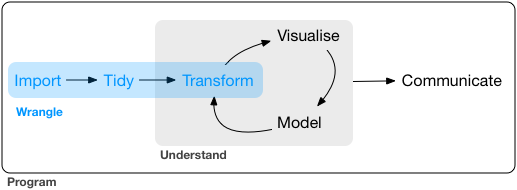
Data wrangling sometimes is also referred to as data munging. It is the process of transforming and mapping data from one “raw” data form into another format to make it more appropriate and valuable for various downstream purposes such as analytics. The goal of data wrangling is to ensure quality and valuable data. Data analysts typically spend the majority of their time in the process of data wrangling compared to the actual analysis of the data. Almost all data require data wrangling before further analysis. There are three main parts to data wrangling (Wickham and Grolemund 2017).
5.3 Data wrangling with dplyr package
5.3.1 dplyr package
dplyr is a package grouped inside tidyverse collection of packages. dplyr package is very useful to munge, wrangle, or transform your data. It is a grammar of data manipulation. It provides a consistent set of verbs that help you solve the most common data manipulation challenges. This tidyverse webpage has more information and examples.
5.3.2 Common data wrangling processes
The common data wrangling processes include:
- reducing the size of dataset by selecting certain variables (or columns)
- generating new variable from existing variables
- sorting observation of a variable
- grouping observations based on certain criteria
- reducing variables to groups in order to estimate summary statistic
5.3.3 Some dplyr functions
For the procedures listed above, the corresponding dplyr functions are
dplyr::select()- to select a number of variables from a dataframedplyr::mutate()- to generate a new variable from existing variablesdplyr::arrange()- to sort observation of a variabledplyr::filter()- to group observations that fulfil certain criteriadplyr::group_by()anddplyr::summarize()- to reduce variable to groups in order to provide summary statistic
5.4 Preparation
5.4.1 Create a new project or set the working directory
It is essential to ensure you know where your working directory is. The recommended practice is to create a new project every time you want to start a new analysis with R. To do so, create a new project by File -> New Project. If you do not start with an R new project, you still need to know the location of your working directory on your computer.
So, again we emphasize that every time you want to start processing your data, please make sure:
- use R project. It is much easier and cleaner to start your work with a new R project. Once you have done or need to log off your computer, close the project and reopen the project the next time you need to.
- if you are not using R project, you are inside the correct working directory. Type
getwd()to display the active working directory. And to set a new working directory, use the functionsetwd(). Once you know where your working directory is, you can start reading or importing data into your working directory.
Once inside the project, you can import your data if necessary.
5.4.2 Load the libraries
Remember, there are several packages you can use to read the data into R. R can read almost all (if not all format) types of data format. For example, we know that common data formats are the:
- SPSS (
.sav) format, - Stata (
.dta) format, - SAS format,
- MS Excel (
.xlsx) format - Comma-separated-values
.csvformat.
However, there are other formats, too, such as data in DICOM format. DICOM format data includes data from CT scans and MRI images. There are data in shapefile format to store geographical information. Three packages - haven, rio, readr and foreign packages - are very useful to read or import your data into R memory.
- readr provides a fast and friendly way to read rectangular data (like csv, tsv, and fwf). This is contained inside the tidyverse metapackage
- rio provides a quick way to read almost all type of spreadsheet and statistical software data
- readxl reads .xls and .xlsx sheets.
- haven reads SPSS, Stata, and SAS data.
We will use the here package to facilitate us working with the working directory and lubridate to help us wrangle dates.
## ── Attaching core tidyverse packages ──────────────────────── tidyverse 2.0.0 ──
## ✔ dplyr     1.1.4     ✔ readr     2.1.5
## ✔ forcats   1.0.0     ✔ stringr   1.5.1
## ✔ ggplot2   3.5.1     ✔ tibble    3.2.1
## ✔ lubridate 1.9.3     ✔ tidyr     1.3.1
## ✔ purrr     1.0.2
## ── Conflicts ────────────────────────────────────────── tidyverse_conflicts() ──
## ✖ dplyr::filter() masks stats::filter()
## ✖ dplyr::lag()    masks stats::lag()
## ℹ Use the conflicted package (<http://conflicted.r-lib.org/>) to force all conflicts to become errors## here() starts at D:/Data_Analysis_CRC_multivar_data_analysis_codesWhen we read datasets with long variable names and spaces - especially after reading the MS Excel dataset - we can use the janitor package to generate more R user-friendly variable names.
5.4.3 Datasets
We will use two datasets.
- the stroke dataset in
csvformat - the peptic ulcer dataset in
xlsxformat
Let’s read the datasets and name it, each as
- stroke
- pep
## Rows: 213 Columns: 12
## ── Column specification ────────────────────────────────────────────────────────
## Delimiter: ","
## chr (7): doa, dod, status, sex, dm, stroke_type, referral_from
## dbl (5): gcs, sbp, dbp, wbc, time2
##
## ℹ Use `spec()` to retrieve the full column specification for this data.
## ℹ Specify the column types or set `show_col_types = FALSE` to quiet this message.Take a peek at the stroke and pep datasets.
The stroke dataset contains:
- 219 observations
- 12 variables
## Rows: 213
## Columns: 12
## $ doa           <chr> "17/2/2011", "20/3/2011", "9/4/2011", "12/4/2011", "12/4…
## $ dod           <chr> "18/2/2011", "21/3/2011", "10/4/2011", "13/4/2011", "13/…
## $ status        <chr> "alive", "alive", "dead", "dead", "alive", "dead", "aliv…
## $ sex           <chr> "male", "male", "female", "male", "female", "female", "m…
## $ dm            <chr> "no", "no", "no", "no", "yes", "no", "no", "yes", "yes",…
## $ gcs           <dbl> 15, 15, 11, 3, 15, 3, 11, 15, 6, 15, 15, 4, 4, 10, 12, 1…
## $ sbp           <dbl> 151, 196, 126, 170, 103, 91, 171, 106, 170, 123, 144, 23…
## $ dbp           <dbl> 73, 123, 78, 103, 62, 55, 80, 67, 90, 83, 89, 120, 120, …
## $ wbc           <dbl> 12.5, 8.1, 15.3, 13.9, 14.7, 14.2, 8.7, 5.5, 10.5, 7.2, …
## $ time2         <dbl> 1, 1, 1, 1, 1, 1, 1, 1, 1, 1, 1, 1, 1, 1, 1, 1, 1, 1, 1,…
## $ stroke_type   <chr> "IS", "IS", "HS", "IS", "IS", "HS", "IS", "IS", "HS", "I…
## $ referral_from <chr> "non-hospital", "non-hospital", "hospital", "hospital", …
The pep datasets contains:
- 121 observations
- 34 variables
## Rows: 121
## Columns: 34
## $ age                 <dbl> 42, 66, 67, 19, 77, 39, 62, 71, 69, 97, 52, 21, 57…
## $ gender              <chr> "male", "female", "male", "male", "male", "male", …
## $ epigastric_pain     <chr> "yes", "yes", "yes", "yes", "yes", "yes", "yes", "…
## $ vomiting            <chr> "no", "no", "no", "no", "yes", "no", "no", "yes", …
## $ nausea              <chr> "no", "no", "no", "no", "yes", "no", "no", "no", "…
## $ fever               <chr> "no", "no", "no", "no", "no", "yes", "no", "yes", …
## $ diarrhea            <chr> "no", "no", "yes", "no", "no", "no", "no", "yes", …
## $ malena              <chr> "no", "no", "no", "no", "no", "no", "no", "no", "n…
## $ onset_more_24_hrs   <chr> "no", "no", "no", "yes", "yes", "yes", "yes", "no"…
## $ NSAIDS              <chr> "no", "no", "yes", "no", "no", "no", "no", "no", "…
## $ septic_shock        <chr> "no", "no", "no", "no", "no", "no", "no", "no", "n…
## $ previous_OGDS       <chr> "no", "no", "no", "yes", "no", "no", "no", "no", "…
## $ ASA                 <dbl> 1, 1, 1, 1, 2, 1, 2, 2, 1, 1, 2, 1, 2, 1, 1, 2, 2,…
## $ systolic            <dbl> 141, 197, 126, 90, 147, 115, 103, 159, 145, 105, 1…
## $ diastolic           <dbl> 98, 88, 73, 40, 82, 86, 55, 68, 75, 65, 74, 50, 86…
## $ inotropes           <chr> "no", "no", "no", "no", "no", "no", "no", "no", "n…
## $ pulse               <dbl> 109, 126, 64, 112, 89, 96, 100, 57, 86, 100, 109, …
## $ tenderness          <chr> "generalized", "generalized", "generalized", "loca…
## $ guarding            <chr> "yes", "yes", "yes", "yes", "no", "yes", "yes", "n…
## $ hemoglobin          <dbl> 18.0, 12.0, 12.0, 12.0, 11.0, 18.0, 8.1, 13.3, 11.…
## $ twc                 <dbl> 6.0, 6.0, 13.0, 20.0, 21.0, 4.0, 5.0, 12.0, 6.0, 2…
## $ platelet            <dbl> 415, 292, 201, 432, 324, 260, 461, 210, 293, 592, …
## $ creatinine          <dbl> 135, 66, 80, 64, 137, 102, 69, 92, 94, 104, 58, 24…
## $ albumin             <chr> "27", "28", "32", "42", "38", "38", "30", "41", "N…
## $ PULP                <dbl> 2, 3, 3, 2, 7, 1, 2, 5, 3, 4, 2, 3, 4, 3, 5, 5, 1,…
## $ admission_to_op_hrs <dbl> 2, 2, 3, 3, 3, 3, 4, 4, 4, 4, 4, 5, 5, 6, 6, 6, 6,…
## $ perforation         <dbl> 0.5, 1.0, 0.5, 0.5, 1.0, 1.0, 3.0, 1.5, 0.5, 1.5, …
## $ degree_perforation  <chr> "small", "small", "small", "small", "small", "smal…
## $ side_perforation    <chr> "distal stomach", "distal stomach", "distal stomac…
## $ ICU                 <chr> "no", "no", "no", "no", "yes", "no", "yes", "no", …
## $ SSSI                <chr> "no", "no", "no", "no", "no", "no", "no", "no", "n…
## $ anast_leak          <chr> "no", "no", "no", "no", "no", "no", "no", "no", "n…
## $ sepsis              <chr> "no", "no", "no", "no", "no", "no", "yes", "no", "…
## $ outcome             <chr> "alive", "alive", "alive", "alive", "alive", "aliv…
Next, we examine the first five observations of the data. The rest of the observations are not shown. You can also see the types of variables:
chr(character),int(integer),dbl(double)
## # A tibble: 5 × 12
##   doa       dod     status sex   dm      gcs   sbp   dbp   wbc time2 stroke_type
##   <chr>     <chr>   <chr>  <chr> <chr> <dbl> <dbl> <dbl> <dbl> <dbl> <chr>
## 1 17/2/2011 18/2/2… alive  male  no       15   151    73  12.5     1 IS
## 2 20/3/2011 21/3/2… alive  male  no       15   196   123   8.1     1 IS
## 3 9/4/2011  10/4/2… dead   fema… no       11   126    78  15.3     1 HS
## 4 12/4/2011 13/4/2… dead   male  no        3   170   103  13.9     1 IS
## 5 12/4/2011 13/4/2… alive  fema… yes      15   103    62  14.7     1 IS
## # ℹ 1 more variable: referral_from <chr>## age gender epigastric_pain vomiting nausea fever diarrhea malena
## 1 42 male yes no no no no no
## 2 66 female yes no no no no no
## 3 67 male yes no no no yes no
## 4 19 male yes no no no no no
## 5 77 male yes yes yes no no no
## onset_more_24_hrs NSAIDS septic_shock previous_OGDS ASA systolic diastolic
## 1 no no no no 1 141 98
## 2 no no no no 1 197 88
## 3 no yes no no 1 126 73
## 4 yes no no yes 1 90 40
## 5 yes no no no 2 147 82
## inotropes pulse tenderness guarding hemoglobin twc platelet creatinine
## 1 no 109 generalized yes 18 6 415 135
## 2 no 126 generalized yes 12 6 292 66
## 3 no 64 generalized yes 12 13 201 80
## 4 no 112 localized yes 12 20 432 64
## 5 no 89 generalized no 11 21 324 137
## albumin PULP admission_to_op_hrs perforation degree_perforation
## 1 27 2 2 0.5 small
## 2 28 3 2 1.0 small
## 3 32 3 3 0.5 small
## 4 42 2 3 0.5 small
## 5 38 7 3 1.0 small
## side_perforation ICU SSSI anast_leak sepsis outcome
## 1 distal stomach no no no no alive
## 2 distal stomach no no no no alive
## 3 distal stomach no no no no alive
## 4 distal stomach no no no no alive
## 5 distal stomach yes no no no alive5.5 Select variables, generate new variable and rename variable
We will work with these functions.
dplyr::select()dplyr::mutate()anddplyr::rename()
5.5.1 Select variables using dplyr::select()
When you work with large datasets with many columns, it is sometimes easier to select only the necessary columns to reduce the dataset size. This is possible by creating a smaller dataset (fewer variables). Then you can work on the initial part of data analysis with this smaller dataset. This will greatly help data exploration.
To create smaller datasets, select some of the columns (variables) in the dataset. For example, in pep data, we have 34 variables. Let us generate a new dataset named pep2 with only ten variables ,
pep2 <- pep %>%
  dplyr::select(age, systolic, diastolic, perforation, twc,
                              gender, vomiting, malena, ASA, outcome)
glimpse(pep2)
## Rows: 121
## Columns: 10
## $ age <dbl> 42, 66, 67, 19, 77, 39, 62, 71, 69, 97, 52, 21, 57, 58, 84…
## $ systolic <dbl> 141, 197, 126, 90, 147, 115, 103, 159, 145, 105, 113, 92, …
## $ diastolic <dbl> 98, 88, 73, 40, 82, 86, 55, 68, 75, 65, 74, 50, 86, 65, 50…
## $ perforation <dbl> 0.5, 1.0, 0.5, 0.5, 1.0, 1.0, 3.0, 1.5, 0.5, 1.5, 1.0, 0.5…
## $ twc <dbl> 6.0, 6.0, 13.0, 20.0, 21.0, 4.0, 5.0, 12.0, 6.0, 28.0, 11.…
## $ gender <chr> "male", "female", "male", "male", "male", "male", "female"…
## $ vomiting <chr> "no", "no", "no", "no", "yes", "no", "no", "yes", "no", "n…
## $ malena <chr> "no", "no", "no", "no", "no", "no", "no", "no", "no", "no"…
## $ ASA <dbl> 1, 1, 1, 1, 2, 1, 2, 2, 1, 1, 2, 1, 2, 1, 1, 2, 2, 1, 1, 3…
## $ outcome <chr> "alive", "alive", "alive", "alive", "alive", "alive", "dea…The new dataset pep2 is now created. You can see it in the Environment pane.
5.5.2 Generate new variable using mutate()
With mutate(), you can generate a new variable. For example, in the dataset pep2, we want to create a new variable named pulse_pressure (systolic minus diastolic blood pressure in mmHg).
\[pulse \: pressure = systolic \: BP - diastolic \: BP \]
And let’s observe the first five observations:
pep2 <- pep2 %>%
  mutate(pulse_pressure = systolic - diastolic)
pep2 %>%
  dplyr::select(systolic, diastolic, pulse_pressure ) %>%
  slice_head(n = 5)
## systolic diastolic pulse_pressure
## 1 141 98 43
## 2 197 88 109
## 3 126 73 53
## 4 90 40 50
## 5 147 82 65Now for the stroke dataset, we will convert doa and dod, both character variables, to a variable of the date type
## # A tibble: 213 × 12
##    doa        dod        status sex    dm      gcs   sbp   dbp   wbc time2
##    <date>     <date>     <chr>  <chr>  <chr> <dbl> <dbl> <dbl> <dbl> <dbl>
##  1 2011-02-17 2011-02-18 alive  male   no       15   151    73  12.5     1
##  2 2011-03-20 2011-03-21 alive  male   no       15   196   123   8.1     1
##  3 2011-04-09 2011-04-10 dead   female no       11   126    78  15.3     1
##  4 2011-04-12 2011-04-13 dead   male   no        3   170   103  13.9     1
##  5 2011-04-12 2011-04-13 alive  female yes      15   103    62  14.7     1
##  6 2011-05-04 2011-05-05 dead   female no        3    91    55  14.2     1
##  7 2011-05-22 2011-05-23 alive  male   no       11   171    80   8.7     1
##  8 2011-05-23 2011-05-24 alive  female yes      15   106    67   5.5     1
##  9 2011-07-11 2011-07-12 dead   female yes       6   170    90  10.5     1
## 10 2011-09-04 2011-09-05 alive  female no       15   123    83   7.2     1
## # ℹ 203 more rows
## # ℹ 2 more variables: stroke_type <chr>, referral_from <chr>5.6 Sorting data and selecting observation
The function arrange() can sort the data. And the function filter() allows you to select observations based on your criteria.
5.6.1 Sorting data using arrange()
We can sort data in ascending or descending order using the arrange() function. For example, for dataset stroke, let us sort the doa from the earliest.
## # A tibble: 213 × 12
##    doa        dod        status sex    dm      gcs   sbp   dbp   wbc time2
##    <date>     <date>     <chr>  <chr>  <chr> <dbl> <dbl> <dbl> <dbl> <dbl>
##  1 2011-01-01 2011-01-05 dead   female yes      15   150    87  12.5     4
##  2 2011-01-03 2011-01-06 alive  male   no       15   152   108   7.4     3
##  3 2011-01-06 2011-01-22 alive  female yes      15   231   117  22.4    16
##  4 2011-01-16 2011-02-08 alive  female no       11   110    79   9.6    23
##  5 2011-01-18 2011-01-23 alive  male   no       15   199   134  18.7     5
##  6 2011-01-20 2011-01-24 dead   female no        7   190   101  11.3     4
##  7 2011-01-25 2011-02-16 alive  female yes       5   145   102  15.8    22
##  8 2011-01-28 2011-02-11 dead   female yes      13   161    96   8.5    14
##  9 2011-01-29 2011-02-02 alive  male   no       15   222   129   9       4
## 10 2011-01-31 2011-02-02 alive  male   no       15   161   107   9.5     2
## # ℹ 203 more rows
## # ℹ 2 more variables: stroke_type <chr>, referral_from <chr>
5.6.2 Select observation using filter()
We use the filter() function to select observations based on certain criteria. Here, in this example, we will create a new dataset (which we will name as stroke_m_40) that contains patients that have sex as male and Glasgow Coma Scale (gcs) at 7 or higher:
- gender is male
- gcs at 7 or higher
## # A tibble: 85 × 12
##    doa        dod        status sex   dm      gcs   sbp   dbp   wbc time2
##    <date>     <date>     <chr>  <chr> <chr> <dbl> <dbl> <dbl> <dbl> <dbl>
##  1 2011-02-17 2011-02-18 alive  male  no       15   151    73  12.5     1
##  2 2011-03-20 2011-03-21 alive  male  no       15   196   123   8.1     1
##  3 2011-05-22 2011-05-23 alive  male  no       11   171    80   8.7     1
##  4 2011-11-28 2011-11-29 dead   male  no       10   207   128  10.8     1
##  5 2012-02-22 2012-02-23 dead   male  no        7   150    80  15.5     1
##  6 2012-03-25 2012-03-26 alive  male  no       14   128    79  10.3     1
##  7 2012-04-02 2012-04-03 alive  male  no       15   143    59   7.1     1
##  8 2011-01-31 2011-02-02 alive  male  no       15   161   107   9.5     2
##  9 2011-02-06 2011-02-08 alive  male  no       15   153    61  11.2     2
## 10 2011-02-20 2011-02-22 alive  male  no       15   143    93  15.6     2
## # ℹ 75 more rows
## # ℹ 2 more variables: stroke_type <chr>, referral_from <chr>
Next, we will create a new dataset (named stroke_high_BP) that contain
sbpabove 130 ORdbpabove 90
## # A tibble: 173 × 12
##    doa        dod        status sex    dm      gcs   sbp   dbp   wbc time2
##    <date>     <date>     <chr>  <chr>  <chr> <dbl> <dbl> <dbl> <dbl> <dbl>
##  1 2011-02-17 2011-02-18 alive  male   no       15   151    73  12.5     1
##  2 2011-03-20 2011-03-21 alive  male   no       15   196   123   8.1     1
##  3 2011-04-12 2011-04-13 dead   male   no        3   170   103  13.9     1
##  4 2011-05-22 2011-05-23 alive  male   no       11   171    80   8.7     1
##  5 2011-07-11 2011-07-12 dead   female yes       6   170    90  10.5     1
##  6 2011-10-12 2011-10-13 alive  female no       15   144    89   5.7     1
##  7 2011-10-21 2011-10-22 alive  male   no        4   230   120  12.7     1
##  8 2011-10-26 2011-10-27 dead   female no        4   207   120  16.5     1
##  9 2011-11-28 2011-11-29 dead   male   no       10   207   128  10.8     1
## 10 2011-12-29 2011-12-30 alive  female no       12   178   100   8.8     1
## # ℹ 163 more rows
## # ℹ 2 more variables: stroke_type <chr>, referral_from <chr>
5.7 Group data and get summary statistics
Thegroup_by() function allows us to group data based on categorical variable. Using the summarize we do summary statistics for the overall data or for groups created using group_by() function.
5.7.1 Group data using group_by()
The group_by function will prepare the data for group analysis. For example,
- to get summary values for mean
sbp, meandbpand meangcs - for sex
5.7.2 Summary statistic using summarize()
Now that we have a group data named stroke_sex, now, we would summarize our data using the mean and standard deviation (SD) for the groups specified above.
stroke_sex %>%
  summarise(meansbp = mean(sbp, na.rm = TRUE),
            meandbp  = mean(dbp, na.rm = TRUE),
            meangcs = mean(gcs, na.rm = TRUE))
## # A tibble: 2 × 4
## sex meansbp meandbp meangcs
## <chr> <dbl> <dbl> <dbl>
## 1 female 166. 91.5 11.9
## 2 male 159. 91.6 13.3To calculate the frequencies for two variables for pep dataset
- sex
- outcome
## # A tibble: 4 × 3
## # Groups:   sex [2]
##   sex    outcome     n
##   <chr>  <chr>   <int>
## 1 male   alive      70
## 2 male   dead       26
## 3 female alive      13
## 4 female dead       12
or
##      sex outcome  n
## 1   male   alive 70
## 2   male    dead 26
## 3 female   alive 13
## 4 female    dead 12
5.8 More complicated dplyr verbs
To be more efficient, use multiple dplyr (a package inside tidyverse meta-package) functions in one line of R code. For example,
pep2 %>%
  filter(sex == "male", diastolic >= 60, systolic >= 80) %>%
  dplyr::select(age, systolic, diastolic, perforation, outcome) %>%
  group_by(outcome) %>%
  summarize(mean_sbp = mean(systolic, na.rm = TRUE),
            mean_dbp = mean(diastolic, na.rm = TRUE),
            mean_perf = mean(perforation, na.rm = TRUE),
            freq = n())
## # A tibble: 2 × 5
## outcome mean_sbp mean_dbp mean_perf freq
## <chr> <dbl> <dbl> <dbl> <int>
## 1 alive 135. 77.2 0.920 61
## 2 dead 130. 75.5 1.80 235.9 Data transformation for categorical variables
5.9.1 forcats package
Data transformation for categorical variables (factor variables) can be facilitated using the forcats package.
5.9.2 Conversion from numeric to factor variables
Now, we will convert the integer (numerical) variable to a factor (categorical) variable. For example, we will generate a new factor (categorical) variable named high_bp from variables sbp and dbp (both double variables). We will label high_bpas High or Not High.
The criteria:
- if sbp \(sbp \geq 130\) or \(dbp \geq 90\) then labelled as High, else is Not High
stroke <- stroke %>%
  mutate(high_bp = if_else(sbp >= 130 | dbp >= 90,
                           "High", "Not High"))
stroke %>% count(high_bp)
## # A tibble: 2 × 2
## high_bp n
## <chr> <int>
## 1 High 177
## 2 Not High 36of by using cut()
stroke <- stroke %>%
  mutate(cat_sbp = cut(sbp, breaks = c(-Inf, 120, 130, Inf),
                       labels = c('<120', '121-130', '>130')))
stroke %>% count(cat_sbp)
## # A tibble: 3 × 2
## cat_sbp n
## <fct> <int>
## 1 <120 25
## 2 121-130 16
## 3 >130 172## # A tibble: 3 × 3
## cat_sbp minsbp maxsbp
## <fct> <dbl> <dbl>
## 1 <120 75 120
## 2 121-130 122 130
## 3 >130 132 2905.9.3 Recoding variables
We use this function to recode variables from old to new levels. For example:
stroke <- stroke %>%
  mutate(cat_sbp2 = recode(cat_sbp, "<120" = "120 or less",
                          "121-130" = "121 to 130",
                          ">130" = "131 or higher"))
stroke %>% count(cat_sbp2)
## # A tibble: 3 × 2
## cat_sbp2 n
## <fct> <int>
## 1 120 or less 25
## 2 121 to 130 16
## 3 131 or higher 1725.9.4 Changing the level of categorical variable
Variable cat_sbp will be ordered as
- less or 120, then
- 121 - 130, then
- 131 or higher
## [1] "<120" "121-130" ">130"## # A tibble: 3 × 2
## cat_sbp n
## <fct> <int>
## 1 <120 25
## 2 121-130 16
## 3 >130 172To change the order (in reverse for example), we can use fct_relevel. Below the first level group is sbp above 130, followed by 121 to 130 and the highest group is less than 120.
stroke <- stroke %>%
  mutate(relevel_cat_sbp = fct_relevel(cat_sbp, ">130", "121-130", "<120"))
levels(stroke$relevel_cat_sbp)
## [1] ">130" "121-130" "<120"## # A tibble: 3 × 2
## relevel_cat_sbp n
## <fct> <int>
## 1 >130 172
## 2 121-130 16
## 3 <120 255.10 Additional resources
The link to webpages below helps readers explore more about Data transformation or wrangling using R.
5.11 Summary
dplyr package is a very useful package that encourages users to use proper verb when manipulating variables (columns) and observations (rows). We have learned to use five functions but there are more functions available. Other useful functions include dplyr::distinct(), dplyr::transmutate(), dplyr::sample_n() and dplyr::sample_frac(). If you are working with a database, you can use dbplyr, which performs data wrangling very effectively with databases. For categorical variables, you can use forcats package.