3.2 PCA to measure SEP
Now we will run a PCA, following Vyas et al (2004), assuming that the first principal component can be used as a measure of socioeconomic position. Again, to unpack what’s going on behind this code, it may be worth revisiting the beers example from the lecture - the associated Rmd file can also be found on Daniel’s github.
Note that we have to manually recode each categorical variable into a binary variable - dummy_cols() handles this for us in R! We also have to manually remove any individuals with missing data - we do not here take a principled approach to missing data, we will simply remove it and assume that it is missing completely at random. Depending on the degree of missing data, this would normally not be the appropriate approach! Note how many individuals were lost when we removed rows containing missing data.
#--- Remove missing data
assets <- assets %>% drop_na()

#--- Create dummy columns
dummies <- assets %>% select(water, floor, wall, roof) %>% dummy_cols() %>%
  select(-c(water, floor, wall, roof))

#--- Convert the remaining data into numeric variables for analysis
cols <- assets %>% select(electricity, radio, tv, fridge, car, toilet) %>% mutate_all(as.numeric) - 1

#--- Bind the dummy columns back together with the other variables
pca_cols <- cbind(cols, dummies)

#--- Conduct the PCA
assets_pca <- prcomp(pca_cols, scale = T)

#--- Get the eigenvectors for PC1-PC3
assets_pca$rotation[,1:3] %>% round(2)
## PC1 PC2 PC3
## electricity 0.33 -0.26 0.15
## radio 0.15 0.03 -0.07
## tv 0.30 -0.27 0.15
## fridge 0.27 -0.27 0.19
## car 0.15 -0.15 0.07
## toilet 0.12 -0.15 -0.37
## water_Protected well -0.03 -0.06 -0.26
## water_Open Well -0.10 -0.10 0.11
## water_Stream, river, lake, other -0.09 -0.21 -0.23
## water_Piped to dwelling 0.29 -0.14 0.11
## water_Piped to local source 0.02 0.42 0.20
## floor_earth, sand -0.36 -0.14 0.05
## floor_cement 0.34 0.18 -0.08
## floor_carpet 0.10 -0.13 0.08
## floor_other 0.07 -0.14 0.08
## wall_sun-dried bricks -0.13 -0.28 -0.22
## wall_baked bricks 0.01 0.04 -0.46
## wall_cement blocks 0.29 -0.10 0.09
## wall_poles and mud -0.13 0.21 0.48
## wall_stones 0.11 0.17 0.01
## wall_grass -0.03 -0.04 0.05
## wall_wood, timber 0.01 -0.01 -0.02
## roof_grass,thatch,mud -0.30 -0.33 0.19
## roof_iron sheets 0.28 0.35 -0.18
## roof_asbestos, other 0.08 -0.10 0.00#--- Get the eigenvalues (and Proportion of Variance)
summary(assets_pca)## Importance of components:
## PC1 PC2 PC3 PC4 PC5 PC6 PC7
## Standard deviation 2.231 1.4726 1.360 1.1782 1.1353 1.1025 1.0745
## Proportion of Variance 0.199 0.0867 0.074 0.0555 0.0515 0.0486 0.0462
## Cumulative Proportion 0.199 0.2858 0.360 0.4153 0.4669 0.5155 0.5617
## PC8 PC9 PC10 PC11 PC12 PC13 PC14
## Standard deviation 1.0380 1.0231 1.0062 0.9981 0.9588 0.949 0.9440
## Proportion of Variance 0.0431 0.0419 0.0405 0.0398 0.0368 0.036 0.0356
## Cumulative Proportion 0.6048 0.6467 0.6872 0.7270 0.7638 0.800 0.8355
## PC15 PC16 PC17 PC18 PC19 PC20 PC21
## Standard deviation 0.9036 0.8821 0.8446 0.7892 0.725 0.6281 0.5127
## Proportion of Variance 0.0327 0.0311 0.0285 0.0249 0.021 0.0158 0.0105
## Cumulative Proportion 0.8681 0.8992 0.9278 0.9527 0.974 0.9895 1.0000
## PC22 PC23
## Standard deviation 0.0000000000000168 0.00000000000000941
## Proportion of Variance 0.0000000000000000 0.00000000000000000
## Cumulative Proportion 1.0000000000000000 1.00000000000000000
## PC24 PC25
## Standard deviation 0.00000000000000902 0.00000000000000691
## Proportion of Variance 0.00000000000000000 0.00000000000000000
## Cumulative Proportion 1.00000000000000000 1.00000000000000000(assets_pca$sdev)^2 %>% round(2)## [1] 4.98 2.17 1.85 1.39 1.29 1.22 1.15 1.08 1.05 1.01 1.00 0.92 0.90 0.89
## [15] 0.82 0.78 0.71 0.62 0.53 0.39 0.26 0.00 0.00 0.00 0.00Let’s extract the eigenvectors (loadings) first. ‘Loadings’ is a term used to refer to the eigenvectors when they are transformed by multiplication by the square root of the eigenvalues and it is actually ‘loadings’ that prcomp() returns. Mathematically, this is done such that the loadings can be interpreted directly as the correlation between the component and the variable. Untransformed eigenvectors themselves are not useful for interpretation of a PCA - I use the two terms ‘eigenvector’ and ‘loading’ interchangeably although this is not strictly correct…!
How many principal components did the PCA produce? What proportion of the total variance is explained by the first prinipal component? The second?
Which variables are associated with Principal Component 1?
We can interpret the loadings as the correlation between the principal component and the variable - so we can see that electricity access, TV ownership, fridge ownership, having water piped to the house, and having floors and walls made of cement are associated with high values of PC1 (ascertained from the positive sign of the eigenvector, indicating a positive correlation). Having a floor made of earth or sand and a roof made of grass, thatch, or mud are associated with low values of PC1.
Do these associations make sense with your initial suggestions about which assets or household characteristics would be associated with higher socioeconomic position?
Let’s now assume that PC1 is in fact measuring SEP. We can extract the scores for each individual of PC1 and take a look at how the scores are distributed in a plot.
#--- Extract the scores from PC1, where high scores are representative of high SEP
assets$pc1 <- assets_pca$x[,1]

#--- Get a histogram of PC1
ggplot(assets, aes(x = pc1)) +
  geom_histogram(bins = 50)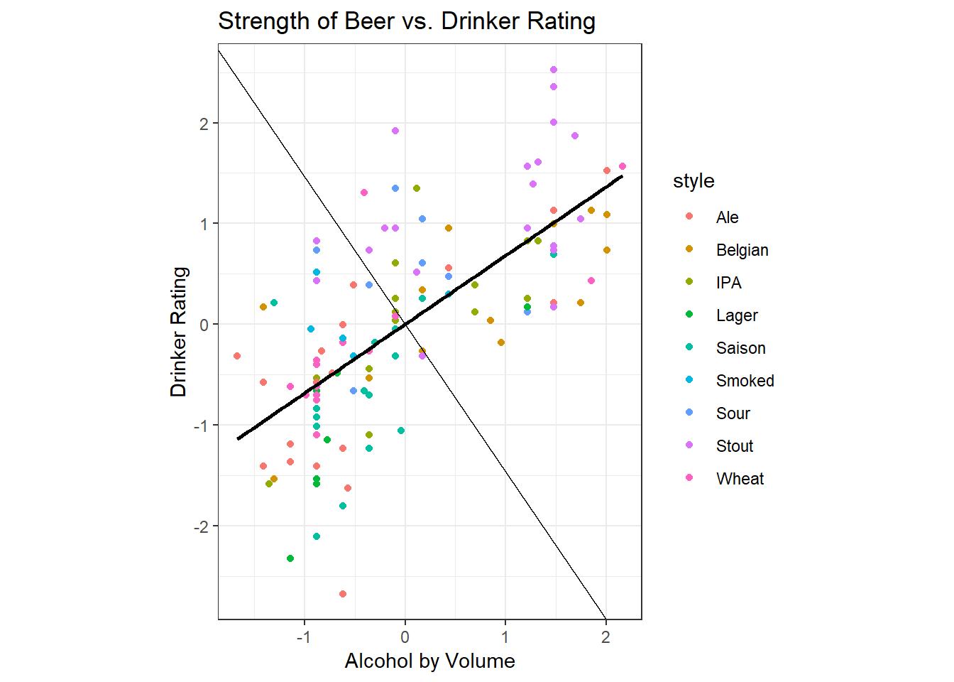
What do you notice about the distribution of the SEP score? Is the SEP score better at distinguishing between low-SEP individuals or high-SEP individuals?
We can either use this score as a continuous variable, but more usually, we divide the score into quintiles.
#--- Generate quintiles
assets <- assets %>% mutate(pc1.q = ntile(pc1, 5)) %>%
                     mutate(pc1.q = as.factor(pc1.q)) %>%
                     mutate(pc1.q = fct_recode(pc1.q,
                                               `Low SEP` = "1",
                                               `Low-Middle SEP` = "2",
                                               `Middle SEP` = "3",
                                               `High-Middle SEP` = "4",
                                               `High SEP` = "5"))

#--- Check quintiles were appropriately created (equal numbers in each group)
summary(assets$pc1.q)
## Low SEP Low-Middle SEP Middle SEP High-Middle SEP
## 549 548 548 548
## High SEP
## 548#--- Get the mean score in each quintile
assets %>% group_by(pc1.q) %>% dplyr::summarise(mean = mean(pc1))## # A tibble: 5 x 2
## pc1.q mean
## <fct> <dbl>
## 1 Low SEP -1.91
## 2 Low-Middle SEP -1.55
## 3 Middle SEP -0.717
## 4 High-Middle SEP 0.521
## 5 High SEP 3.66Now we have two distinct measures of SEP: we have an asset/household characteristic index and we also have education, which in many contexts, is part of socioeconomic position.