1.5 Biplots and Interpretation
It can be made clear by means of a biplot that graphically displays the results of the PCA.
ggbiplot(beers_pca, obs.scale = 1, group = beers$style, ellipse = T) +
  scale_color_discrete(name = '') +
  labs(title = "PCA: Beer variables") +
theme_bw() 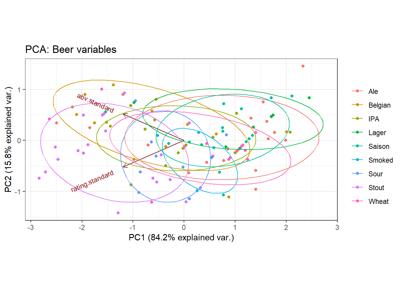
What is this plot telling us? Each variable that went into the PCA has an associated arrow. Arrows for each variable point in the direction of increasing values of that variable.
If you look at the ‘Rating’ arrow, it points towards low values of PC1 - so we know the lower the value of PC1, the higher the Drinker Rating.
If you look at the ‘ABV’ arrow, it also points towards low values of PC1 - so we know the lower the value of PC1, the higher the Alcohol Content.
So we now understand that our summary score that we obtained for each beer, that is, the value of PC1, is lower if a beer is both well-regarded and high in alcohol and higher if a beer is not well-regarded and low in alcohol.
The arrows on the biplot are actually representative of the eigenvectors (loadings), so we could just as easily obtain this information from the matrix of the loadings:
\[\begin{array}{ccc} & PC1 & PC2 \\ ABV & -0.707 & 0.707 \\ Rating & -0.707 & -0.707 \end{array}\]
PC1 is negatively associated with ABV and Rating (the signs of the eigenvectors are negative) and therefore we would expect low values of PC1 to entail high values of ABV & Ratings. PC2 is positively associated with ABV and negatively associated with Rating, so we expect beers with high PC2 scores to be low in alcohol but highly rated.
Note that also from the biplot, we can see that higher ratings are associated with Stout (and not Lager) because the arrow points in the direction of the cluster of Stout points (in purple) and away from the cluster of Lager points (in green). Higher alcohol might be associated with Belgian beers (in orange) and not Wheat beers (in pink).
1.5.1 Extending the Example
What happens if we add some more data into the PCA? Let’s reconduct the PCA and include a new piece of information: the year the beer was released.
#--- Select the new relevant columns
beercols2 <- beers %>% select(abv, rating, year)

#--- Conduct the PCA
beers_pca2 <- prcomp(beercols2, scale = T)

#--- Get the eigenvectors
beers_pca2$rotation
## PC1 PC2 PC3
## abv -0.6502930 0.3121237 -0.69260219
## rating -0.6664807 0.2031397 0.71731286
## year -0.3645854 -0.9280695 -0.07592409#--- Plot the PCA
ggbiplot(beers_pca2, obs.scale = 1, var.scale = 2, group = beers$style, ellipse = T) +
scale_color_discrete(name = '') +
labs(title = "PCA: Beer variables") +
theme_bw() 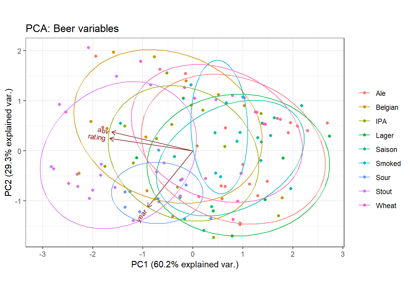
#--- Get the eigenvalues
(beers_pca2$sdev)^2
## [1] 1.8067886 0.8800890 0.3131224#--- Get the proportion of variance (row 2)
summary(beers_pca2)## Importance of components:
## PC1 PC2 PC3
## Standard deviation 1.3442 0.9381 0.5596
## Proportion of Variance 0.6023 0.2934 0.1044
## Cumulative Proportion 0.6023 0.8956 1.0000\[\begin{array}{cccc} & PC1 & PC2 & PC3 \\ ABV & -0.65 & 0.31 & -0.70 \\ Rating & -0.67 & 0.20 & -0.70 \\ Year & -0.37 & -0.93 & -0.08 \end{array}\]
In this case, we see that high values of PC1 are associated with low values of Alcohol Content, low Drinker Rating, and older years. So low values of PC1 are associated with well-regarded beers (loading: -0.65) that are also high in alcohol (loading: -0.67). Low values of PC1 are a little less associated with newness (loading: -0.37). PC1 explains 60.2% of the total variance, making it a fairly good summary measure.
PC2 on the other hand (explaining 29% of the variance), is largely influenced by year (the associated loading is 0.93) - so this implies that there is some aspect of the beer data, independent from being well-regarded and strong, that is explained by the newness of the beer. Note that the composite measure PC2 actually explains less of the variance than any of the given variables (ABV, Rating, Year) alone - since the total variance is 3, each variable alone would explain 33.3% of the variance.