2.2 HIV Prevalence

Now let’s look at the prevalence of HIV in the sample. We can also examine HIV prevalence by age, education, and number of partners using either the tabpct command or the cc command. Use tabpct to get row or column percentages and cc to get an odds ratio and associated confidence interval.

Do you notice any systematic differences in prevalence by these variables?

#--- Stratified summaries of HIV prevalence by Age
tz %$% tabpct(serostat, age.group, percent = "col", graph = F)

## 
## Column percent 
##                age.group
## serostat         14-19       %  20-24       %
##   hiv negative    1569  (99.4)   1134  (95.9)
##   hiv  positive     10   (0.6)     49   (4.1)
##   Total           1579   (100)   1183   (100)

tz %$% cc(serostat, age.group, graph = F)

## 
##                age.group
## serostat        14-19 20-24 Total
##   hiv negative   1569  1134  2703
##   hiv  positive    10    49    59
##   Total          1579  1183  2762
## 
## OR =  6.78 
## 95% CI =  3.42, 13.44  
## Chi-squared = 39.83, 1 d.f., P value = 0
## Fisher's exact test (2-sided) P value = 0

#--- Are there trends in serostatus by age?
tz %>% ggplot(aes(x = as.factor(age), fill = serostat)) +
  geom_bar(position = "dodge")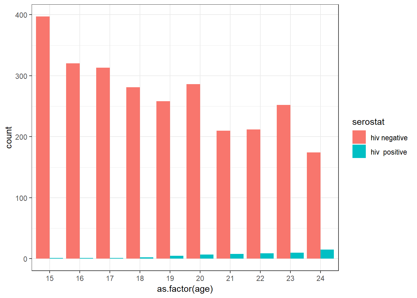

#--- Stratified summaries of HIV prevalence by Education
tz %$% tabpct(educat, serostat, percent = "col", graph = F)

## 
## Column percent 
##                          serostat
## educat                     hiv negative       %  hiv  positive       %
##   no education, preschool           460  (17.0)             18  (30.5)
##   primary                          1743  (64.5)             39  (66.1)
##   secondary                         500  (18.5)              2   (3.4)
##   Total                            2703   (100)             59   (100)

tz %$% cc(serostat, educat, graph = F) 

## 
##                 educat
## serostat         no education, preschool primary secondary
##   hiv negative   460                     1743    500      
##   hiv  positive  18                      39      2        
##                                                           
##   Odds ratio     1                       0.57    0.1      
##   lower 95% CI                           0.32    0.01     
##   upper 95% CI                           1.07    0.43     
## 
## Chi-squared = 13.3 , 2 d.f., P value = 0.001 
## Fisher's exact test (2-sided) P value = 0.001

#--- Stratified summaries of HIV prevalence by Education
tz %$% tabpct(partners.cat, serostat, percent = "row", graph = F)

## 
## Row percent 
##             serostat
## partners.cat  hiv negative  hiv  positive  Total
##           0           1201              2   1203
##                     (99.8)          (0.2)  (100)
##           1            864             18    882
##                       (98)            (2)  (100)
##           2+           636             39    675
##                     (94.2)          (5.8)  (100)

tz %$% cc(partners.cat, serostat, graph = F) 

## 
##             serostat
## partners.cat hiv negative hiv  positive Total
##        0             1201             2  1203
##        1              864            18   882
##        2+             636            39   675
##        Total         2701            59  2760
## 
## OR =  12.51 
## 95% CI =  2.9, 54.06  
## Chi-squared = 65.14, 2 d.f., P value = 0
## Fisher's exact test (2-sided) P value = 0