Chapter 11 Survey data and statistical modeling

The use of survey data in statistical modeling, such as regression analysis, is a common and valuable approach in the fields of economics and finance in order to examine the relationship between one or more independent variables and a dependent variable. Traditional modeling approaches typically assume that the observations are independent and identically distributed. However, when working with survey data these assumptions are often violated and we need to account for complex design features, such as unequal inclusion probabilities, stratification, clustering, reweighting for unit non-response and calibration to external data sources.

11.1 The case of linear regression

In the traditional framework for linear regression, we assume the following linear relationship (M) $Y_i = X_i \beta + \epsilon_i$ between a response variable $Y_i$ and a vector of $p$ explanatory variables $X_i=\left(X^1_i,X^2_i \cdots X^p_i\right)$

$\beta = \left({\beta}_1 , {\beta}_2 \dots {\beta}_p \right)^T$ is the vector of the $p$ model parameters and $\epsilon_i~~\left(i = 1 \cdots n\right)$ are the model residuals, which are assumed to be independent and identically distributed realizations of a normal distribution with mean 0 and variable $\sigma^2$

The vector $\beta$ of model parameters is estimated using the least-squares criterion $Min \sum_{i=1}^n \left(Y_i - X_i B\right)^2$

$$\hat{\beta}_{LS} = \left(\sum_{i=1}^n X_i^T X_i\right)^{-1} \left( \begin{array}{c} \sum_{i=1}^n X^1_i Y_i \\ \\ \sum_{i=1}^n X^2_i Y_i \\ \cdots \\ \sum_{i=1}^n X^p_i Y_i \end{array} \right)$$

$\hat{\beta}_{LS}$ leads to the Best Linear Unbiased Estimator (BLUE) among all the possible linear combinations of the observations.

In the survey settings, in order to take into account complex design features, the parameter $\beta$ is estimated by incorporating the sampling weights $\left( {\omega}_i , i \in s \right)$ into the formula:

$$\hat{\beta}_{\omega} = \left(\sum_{i \in s} \omega_i X_i^T X_i\right)^{-1} \left( \begin{array}{c} \sum_{i \in s} \omega_i X^1_i Y_i \\ \\ \sum_{i \in s} \omega_i X^2_i Y_i \\ \cdots \\ \sum_{i \in s} \omega_i X^p_i Y_i \end{array} \right)$$

In this case, $\hat{\beta}_{\omega}$ is an asymptotically unbiased estimator of the population regression coefficient $B$ under the sampling design:

$$B = \left(\sum_{i \in U} X_i^T X_i\right)^{-1} \left( \begin{array}{c} \sum_{i \in U} X^1_i Y_i \\ \\ \sum_{i \in U} X^2_i Y_i \\ \cdots \\ \sum_{i \in U} X^p_i Y_i \end{array} \right)$$

In contrast to $\beta$, which is a parameter of the regression model, $B$ is finite population parameter. If we consider the population observations as independent, identically distributed realizations of the initial regression model (M) - “super-population” modeling - , $B$ is an unbiased estimator of $\beta$ under the model and its variance is of order $1/N$, which can be neglected as long as the population size is large.

Thus, the estimator $\hat{\beta}_{\omega}$ can be regarded as the result of a “two-phase” process:

• The i.i.d selection of the $N$ population units (“Super-population modeling”): The population regression coefficient $B$ is an unbiased estimator of $\beta$ and its variance is negligible as long as the size $N$ of the population is large
• The selection of the sample $s$ from $U$ according to a sampling plan: the weighted estimator $\hat{\beta}_{\omega}$ is an asymptotically unbiased estimator of $B$ and the design-based variance of $\hat{\beta}_{\omega}$ can be obtained by using the linearization technique. In the case of simple linear regression, the linearised variable of $\hat{\beta}_{\omega}$ is given by:

$$\widetilde{z}_k = \displaystyle{\frac{1}{\hat{N}\hat{\sigma}^2_x}}\left(X_k - \displaystyle{\frac{\hat{X}}{\hat{N}}}\right) \left[\left(Y_k - \displaystyle{\frac{\hat{Y}}{\hat{N}}}\right) - \hat{B} \left(X_k -\displaystyle{\frac{\hat{X}}{\hat{N}}}\right)\right]$$

Therefore, all design features must be taken into account when fitting the model to the data in order to obtain reliable and accurate estimates of the regression coefficients. In particular, the commonly used weighted linear regression, which aims to deal with heteroscedastic errors, i.e. when the errors are heteroskedastic ($V\left(\epsilon_i\right)=\sigma^2_i$), should be discarded as it can only account for unequal sample weights but ignores other design features.

The regression commands in STATA allow this, as long as the keyword svy: is specified at the beginning of the regression command.

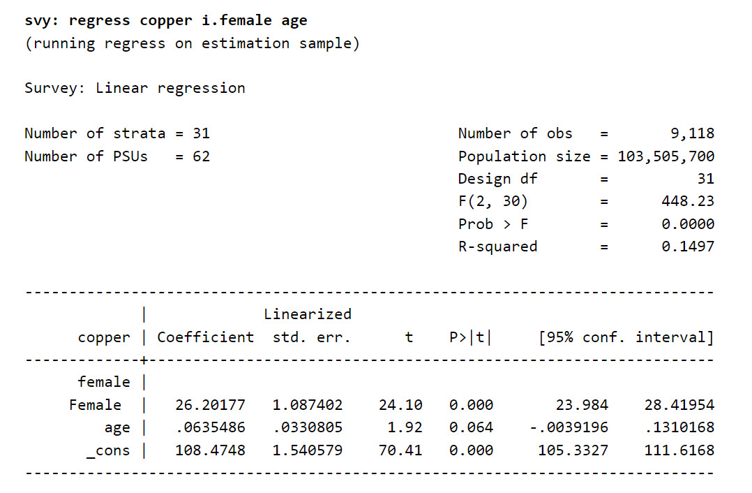
Figure 11.1: Example of a linear regression using the svy command

The output of the regression is similar to that of the traditional i.i.d. regression command. However, there are differences with the output of classical model-based regression, such as

• The number of degrees of freedom, which is based on the number of strata: $df = n - H$, where $df$ is the number of degrees of freedom, $n$ is the number of observations and $H$ is the number of strata.
• The use of “robust” standard error estimators based on linearisation, which take into account all the complex design features.
• The way in which the R-squared coefficient is calculated, taking into account the sample weights.

However, the regression coefficients must be read and interpreted in the same way as in the traditional model-based approach.

11.2 The case of logistic regression

Binary logistic models assume the following relationship between the propensity $p_i$ of a response category and a vector $X_i = \left(X_{1i}, X_{2i} ... X_{Li}\right)^T$ of $L$ predictor variables:

$$p_i = \displaystyle{\frac{e^{A X_i}}{1+e^{A X_i}}}$$

where $A=\left(A_1, A_2 ... A_L\right)$ is the vector of the $L$ model parameters.

Estimation in logistic regression is usually done by maximizing the pseudo-likelihood function:

$$LL = \displaystyle{\prod_{i/y_i=1}\left(\frac{e^{AX_i}}{1+e^{AX_i}}\right)\prod_{j/y_j=0}\left(1-\frac{e^{AX_j}}{1+e^{AX_j}}\right) = \prod_{i}\left(\frac{e^{AX_i}}{1+e^{AX_i}}\right)^{y_i}\left(1-\frac{e^{AX_j}}{1+e^{AX_j}}\right)^{1-y_i}}$$

or, equivalently, by finding the zeros of the derivative of the log pseudo-likelihood function:

$$\begin{equation} \begin{array}{rcl} LogLL & = & \sum_{i} y_i \left[A X_i - Log\left(1+e^{AX_i}\right)\right] + \left(1-y_i\right) \left[0 - Log\left(1+e^{AX_i}\right)\right] \\ & = & \sum_{i} y_i \left(A X_i\right) - Log\left(1+e^{AX_i}\right) \end{array} \end{equation}$$

which is equivalent to solving a system of $L$ equations: $$\displaystyle{\sum_{i} X_{li} \left(y_i - \frac{e^{\hat{A} X_i}}{1+e^{\hat{A} X_i}}\right)} = 0$$

In the survey setting, the corresponding weighted estimator of $A$ is:

$$\displaystyle{\hat{A}_\omega = argmax_{A} \prod_{i \in s/y_i=1} \left(\frac{e^{AX_i}}{1+e^{AX_i}}\right)^{\omega_i} \prod_{j \in s/y_j=0} \left(1-\frac{e^{AX_j}}{1+e^{AX_j}}\right)^{\omega_j}}$$

which is equivalent to solving:

$$\displaystyle{\sum_{i \in s} \omega_i X_{li} \left(y_i - \frac{e^{\hat{A}_\omega X_i}}{1+e^{\hat{A}_\omega X_i}}\right)} = 0$$

11.3 The case of Poisson regression and other regression Models

Poisson regression is commonly used to deal count data. We assume that the number of occurences $y_i$ of an event follows a Poisson distribution $Y_i$ of parameter $\lambda_i$:

$$Pr\left(Y_i=y_i\right) = \displaystyle{e^{-\lambda_i}\frac{\lambda_i^{y_i}}{y_i!}}$$

$\lambda_i$ can be interpreted as the average number of occurences of the event. We assume the following linear relationship between $\lambda_i$ and a vector $X_i = \left(X_{1i}, X_{2i} ... X_{Li}\right)^T$ of $L$ predictor variables:

$$Log\left(\lambda_i\right) = \displaystyle{A_1 X_{1i} + A_2 X_{2i} + ... + A_L X_{Li} = A X_i}$$

As with logistic regression, the model parameters $A=\left(A_1, A_2 ... A_L\right)$ are estimated by maximising the pseudo-likelihood function:

$$LL = \displaystyle{\prod_{i \in s} \left(e^{-\lambda_i}\frac{\lambda_i^{y_i}}{y_i!}\right)^{\omega_i}}$$

or, equivalently, by finding the zeros of the derivative of the log pseudo-likelihood function:

$$LogLL = \displaystyle{\sum_{i \in s} {\omega}_i \left[y_i Log\left(\lambda_i\right)- \lambda_i - Log\left(y_i!\right)\right] = \sum_{i \in s} {\omega}_i \left[y_i \left(A X_i\right) - e^{A X_i} - Log\left(y_i!\right)\right] }$$

which is equivalent to solving a system of $L$ equations: $$\displaystyle{\sum_{i \in s} {\omega}_i X_{li} \left(y_i - e^{\hat{A}_\omega X_i}\right)} = 0$$

This approach to fitting a model based on pseudo-likelihood can be extended to deal with most of the regression-based models encountered in practice, including Generalized Linear Models, sample selection models (e.g. the Heckmann model) or Tobit models for dealing with censored data.

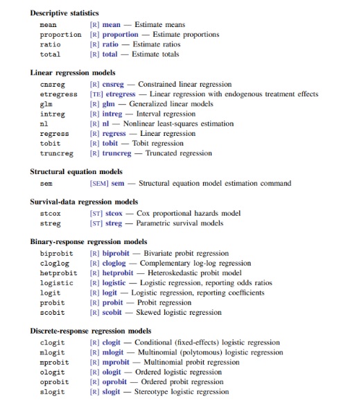
Figure 11.2: Non linear methods supporting the survey commands in STATA

11.4 To weight or not to weight ?

Whether or not to use sample weights in regression analysis is a recurring question to which there is no simple answer.

Weighting is generally seen as a protection against sample bias, so weights should be used when there is a risk that the data are highly biased (unequal inclusion probabilities, stratification, clustering, high non-response, calibration). However, the cost of using weights is an increase in sampling variance.

Therefore, when using models with survey data, it is recommended to test the effect of including weights on the regression results. If the effect on the coefficient estimates is small and the standard errors increase, then the weights have no significant effect. On the other hand, if the difference between unweighted and weighted estimates is important, then the data should be further examined to identify possible inconsistencies or influencing values.

Regardless of the data used, model specification is key and there should be no large differences between weighted and unweighted estimates as long as the model is properly specified. In this case, the use of weights in estimation will lead to increased volatility without any gain in statistical precision.

In summary, the use of survey data in regression analysis requires careful consideration of variable types, sampling methods and potential problems associated with the data. Properly addressing these considerations will increase the reliability and validity of your regression results.