Chapter 3 Stratification

3.1 What is it?

Stratification is a widely used technique in survey sampling, which involves dividing the target population \(U\) into \(H\) non overlapping sub-populations \(U_1, U_2 \cdots U_H\), called strata.

A sample \(s_h\) of size \(n_h\) is taken within each stratum \(h\) independently from one stratum to another. Let \(n = \sum_{h=1}^H n_h\) be the overall sample size.

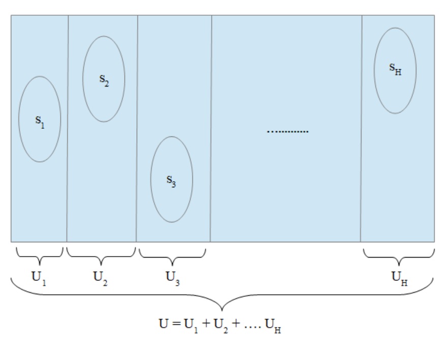
Figure 3.1: Stratification

For instance, we can categorise a population based on age, gender, and city of residence. Similarly, we can classify a frame of enterprises according to criteria such as company size or sector of operation as outlined by the NACE classification.

Stratification is an example of a sampling technique that employs auxiliary information to enhance sampling efficiency. The information is acquired from stratification variables that are known in advance for each unit of the target population.

Stratification is primarily motivated by statistical factors. As demonstrated in the previous chapter that the variability in simple random sampling is dependent on two factors: the sample size (\(n\)) and the dispersion of the variable of interest (\(S^2_y\)). Specifically, a high dispersion (i.e. heavily scattered values) leads to a high variance. Stratification proves effective when the strata are homogeneous for the survey’s study variables. In this scenario, stratification enhances the stability of estimators by reducing their variance.

Additionally, organizational factors may drive stratification whereby a stratum denotes a “regional” office responsible for selecting samples and collecting data in that area.

3.2 Total, mean and proportion estimators

Let \(N_h\) be the size of stratum \(h\). In stratification, the size \(N_h\) is assumed to be known for all strata \(h\). In this situation, the total \(Y\) of a study variable \(y\) can be written as:

\[\begin{equation} Y = \sum_{i \in U} y_i = \sum_{h=1}^{H} \sum_{i \in U_h} y_i = \sum_{h=1}^{H} Y_h = \sum_{h=1}^{H} N_h \bar{Y}_h \tag{3.1} \end{equation}\]

As to the population mean \(\bar{Y}\) of \(y\), it can be expressed as the average of the stratum means \(\bar{Y}_h\) using the ratios \(W_h = N_h/N\) as weights:

\[\begin{equation} \bar{Y} = \sum_{h=1}^{H} \frac{N_h}{N} \bar{Y}_h = \sum_{h=1}^{H} W_h \bar{Y}_h \tag{3.2} \end{equation}\]

Similarly, the proportion \(P\) is determined by weighting the proportions \(P_h\) in each stratum:

\[\begin{equation} P = \sum_{h=1}^{H} \frac{N_h}{N} P_h = \sum_{h=1}^{H} W_h P_h \tag{3.3} \end{equation}\]

Assuming simple random sampling is conducted within each stratum (stratified simple random sampling), unbiased estimators for population totals, means and proportions are given by:

\[\begin{equation} \hat{Y}_{STSRS} = \sum_{h=1}^{H} N_h \bar{y}_h \tag{3.4} \end{equation}\]

\[\begin{equation} \hat{\bar{Y}}_{STSRS} = \sum_{h=1}^{H} W_h \bar{y}_h \tag{3.5} \end{equation}\]

\[\begin{equation} \hat{P}_{STSRS} = \sum_{h=1}^{H} W_h p_h \tag{3.6} \end{equation}\]

In stratified simple random sampling, the design weights are equal within each stratum: \(d_i = N_h/n_h ~~\forall i \in s_h\)

Using the results for simple random sampling, the variances of the three above estimators are:

\[\begin{equation} V\left(\hat{Y}_{STSRS}\right) = \sum_{h=1}^{H} N^2_h \left(1-f_h\right) S^2_h / n_h \tag{3.7} \end{equation}\]

\[\begin{equation} V\left(\hat{\bar{Y}}_{STSRS}\right) = \sum_{h=1}^{H} W^2_h \left(1-f_h\right) S^2_h / n_h \tag{3.8} \end{equation}\]

\[\begin{equation} V\left(\hat{P}_{STSRS}\right) \approx \sum_{h=1}^{H} W^2_h \left(1-f_h\right) P_h\left(1-P_h\right) / n_h \tag{3.9} \end{equation}\]

Assuming the sampling fraction \(f_h\) is the same in each stratum: \(f_h = n_h/N_h = n/N = f ~~\forall h\), we can then rewrite the estimator (3.8) as:

\[\begin{equation} \begin{array}{rcl} V\left(\hat{\bar{Y}}_{STSRS}\right) & = & \sum_{h=1}^{H} W^2_h \left(1-f_h\right) S^2_h / n_h \\ & = & \left(1-f\right) \sum_{h=1}^{H} W^2_h S^2_h / n_h \\ & = & \left(1-f\right) \sum_{h=1}^{H} W_h S^2_h / n \\ & = & \left(1-f\right) S^2_w / n \end{array} \tag{3.10} \end{equation}\]

where \(S^2_w = \sum_{h=1}^{H} W_h S^2_h\) is the within-stratum dispersion.

As \(S^2_w\) is lower than the total population dispersion \(S^2\), it can be shown that:

\[ V\left(\hat{\bar{Y}}_{STSRS}\right) = \left(1-f\right) S^2_w / n \leq \left(1-f\right) S^2 / n = V\left(\hat{\bar{Y}}_{SRS}\right) \] Therefore, stratification leads to mean estimates that are more accurate than those obtained by simple random sampling. The gain in accuracy depends on the ratio \(\rho = S^2_w / S^2\): the more homogeneous the stratum groups are with respect to the variable under study, the better the gain. For example, when conducting a survey on dwelling rents, it is important to stratify the data according to criteria such as geographical location, type of dwelling and area. In a survey of enterprises, the size of the enterprise or the sector of activity (NACE) are important criteria for stratification.

3.3 Sample allocation

Let us assume that the overall sample size \(n\) is predetermined (usually for budgetary reasons). We wish to determine the sample size \(n_h\) to be drawn in each stratum in order to achieve statistical optimality, taking into account budgetary considerations. Various allocation schemes have been proposed in the literature for this purpose.

3.3.1 Equal allocation

In equal allocation, the sample size \(n_h\) is constant across the strata: \[\begin{equation} \forall h~~n^{eq}_h=n/H \tag{3.11} \end{equation}\]

This scheme ensures a minimum level of precision in each stratum. It is thus influenced by local factors. On the other hand, equal allocation performs poorly when it comes to national estimation, especially when the dispersions \(S^2_h\) vary across the different strata.

3.3.2 Proportional allocation

Proportional allocation consists of selecting samples in each stratum in proportion to the size \(N_h\) of the stratum population: \[\begin{equation} \forall h~~n^{prop}_h = n N_h / N = nW_h \tag{3.12} \end{equation}\]

As previously shown, proportional allocation is always more efficient in terms of sample accuracy than simple random sampling of same size \(n\).

\[\begin{equation} V\left(\hat{\bar{Y}}_{prop}\right) = \left(1-f\right)\frac{S^2_w}{n} = \frac{\sum_{h=1}^{H} W_h S^2_h}{n} - \frac{\sum_{h=1}^{H} W_h S^2_h}{N} \tag{3.13} \end{equation}\]

This result justifies the use of stratification as a powerful variance reduction technique.

3.3.3 Optimal allocation

Optimal allocation (also called Neyman allocation) seeks to minimize the variance (3.8) under the cost constraint \(\sum_{h=1}^H c_h n_h = C_0\), where \(C_0\) is the overall budget available and \(c_h\) the average survey cost for an individual in stratum \(h\).

The solution to this problem is given by: \[\begin{equation} \forall h~~n^{opt}_h = \frac{N_h S_h}{\sqrt{c_h}} \frac{C_0}{\sum_{h=1}^H N_h S_h \sqrt{c_h}} \tag{3.14} \end{equation}\]

If there is no cost constraint across the strata (i.e. \(c_h=1~~\forall h\)), then the sample size in stratum \(h\) is: \[\begin{equation} n^{opt}_h = n \frac{N_h S_h}{\sum_{h=1}^H N_h S_h} \tag{3.15} \end{equation}\]

and the variance of (3.8) under Neyman allocation (3.15) is:

\[\begin{equation} \begin{array}{rcl} V\left(\hat{\bar{Y}}_{opt}\right) & = & \displaystyle{\frac{\left(\sum_{h=1}^{H} W_h S_h\right)^2}{n} - \frac{\sum_{h=1}^{H} W_h S^2_h}{N}} \\ & = & \displaystyle{V\left(\hat{\bar{Y}}_{prop}\right) - \frac{1}{n} \sum_h W_h \left(S_h - \bar{S}\right)^2} \\ & = & \displaystyle{V\left(\hat{\bar{Y}}_{SRS}\right) - \frac{1}{n} \sum_h W_h \left(\bar{Y}_h - \bar{Y}\right)^2 - \frac{1}{n} \sum_h W_h \left(S_h - \bar{S}\right)^2} \tag{3.16} \end{array} \end{equation}\]

The Neyman allocation differs from proportional allocation in that it is specifically tailored to a particular study variable. What may be optimal for one variable may not necessarily be optimal for another.

Furthermore, the statistical literature (see e.g. Cochran (1977)) has shown that the increased accuracy gained from using Neyman allocation is generally small. As a result, in practice, proportional allocation tends to be more commonly used than optimal allocation.

3.3.4 Balanced allocation

Both proportional and Neyman allocations improve sample accuracy at a global level, but may exhibit poor performance when estimating region-specific levels. For instance, proportional allocation of a global sample of 5000 individuals would lead to having a sample of 500 individuals when the stratum weight \(W_h\) is equal to 10% of the whole population, and only 100 individuals when the weight is equivalent to 2%.

In order to reconcile local and global considerations, it is advisable to adopt a balanced approach: a subsample \(\tilde{n} \leq n\) may be equally allocated among the strata in order to guarantee minimum accuracy in each group, while the remaining \(n - \tilde{n}\) units may be allocated across the strata by using either proportional or optimal allocations in order to optimize accuracy at global level.

\[\begin{equation} \forall h~~n^{bal}_h = \displaystyle{\frac{\tilde{n}}{H}} + \left(n-\tilde{n}\right) W_h \tag{3.17} \end{equation}\]

In summary, it can be stated that stratification is a firmly established method that benefits both statistical and organisational objectives. That is the reason why it is frequently employed in survey methodology, especially by institutions like STATEC, the National Statistics Institute of Luxembourg.