Survey data in Economics and Finance
2025-01-05
Chapter 1 Introduction
1.1 History
Counting populations through exhaustive censuses has been a practice that has been established for millennia, dating back to the era of ancient civilizations such as the Babylonians, Egyptians and Romans. These populations conducted censuses for supporting a range of economic decisions, including taxation, scaling the labor force, food distribution and industrial investment. Censuses are commonly considered as error-free data sources which yield the most accurate statistics. Conversely, censuses are lengthy and costly endeavours that require a significant amount of time (frequently several years) to plan and execute. As a result, they cannot be conducted at a high frequency. Presently, numerous European nations, such as Luxembourg, conduct population censuses every decade.
To generate updated statistical data between two census periods, sample surveys have proven to be a potent tool. However, the scientific community took a considerable amount of time to validate the concept that gathering data from a population sample may yield result accuracy on par with a census. The recent ascent of survey sampling in contemporary statistical production started in the latter half of the 20th century. This was due to the demonstration that probability theory, notably the Central Limit Theorem, could be applied to calculate accurate confidence intervals and margins of error for survey estimates based on probability samples. This has led to the development of a substantial body of sampling theory, in which Probability and Mathematics are employed to enhance sampling efficiency and enhance the accuracy of data.
Currently, data producers such as national statistics institutes, central banks, public administrations, universities, research centres and private companies frequently employ sample surveys as a pivotal source of statistical data in diverse fields including economy, finance, demography, sociology, environmental research, biology and epidemiology.
1.2 Examples of surveys
In Luxembourg, the National Statistical Institute (STATEC)1 conducts a variety of sample surveys focusing on households, individuals, and businesses within the country.
Example 1: List of all the household surveys conducted by Luxembourg’s STATEC
- Living conditions
- Household Budget Survey
- Safety Survey
- Time Use Survey
- Business and Leisure Tourism Survey
- European Statistics on Income and Living Conditions
- Community Survey on the Usage of Information and Communications Technologies (ICT) among Households and Individuals
- Labour market and education
- Labour Force Survey
- Adult Education Survey
- Population and housing
- Population and Housing Census
- Statistics of Completed Buildings Survey
- Statistics of Transformation Survey
- Price
- Rents Survey
- Housing Characteristics Survey
- Quality
- Confidence in Public Statistics
Central banks are increasingly using survey data as a complement to traditional macroeconomic aggregates. This aids in the monitoring of financial stability, assessing tail risks and studying new policy requirements.
Example 2: List of the surveys supervised by the European Central Bank
- Survey of monetary analysts (SMA)
- ECB survey of professional forecasters (SPF)
- Bank lending survey (BLS)
- Survey on the access to finance of enterprises (SAFE)
- Household finance and consumption survey (HFCS)
- Survey on credit terms and conditions in euro-denominated securities financing and over-the-counter derivatives markets (SESFOD)
- Consumer expectations survey (CES)
Quoting ECB’s website2: “These surveys provide important insights into various issues, such as:
- micro-level information on euro area households’ assets and liabilities
- financing conditions faced by small and medium-sized enterprises
- lending policies of euro area banks
- market participants’ expectations of the future course of monetary policy
- expectations about inflation rates and other macroeconomic variables
- trends in the credit terms offered by firms in the securities financing and over-the-counter (OTC) derivatives markets, and insights into the main drivers of these trends.”
Numerous international survey programs have been established by academic consortiums to explore significant research topics. These studies gather comparable micro-data from the participating nations. For instance, the European Social Survey (ESS)3, the European Values Study (EVS)4, the Survey On Health Ageing and Retirement in Europe (SHARE)5, the International Crime and Victim Survey (ICVS)6, and the Global Monitor Entrepreneurship (GEM)7 are notable examples.
1.3 Pros and cons of surveys
Sample surveys offer faster and more cost-effective results than exhaustive enumerations. This makes them a highly relevant option when statistics are needed quickly and resources in terms of staff, time and money are limited.
In addition, surveys can concentrate on topics that censuses cannot cover in as much detail, such as:
For individuals and households: household income, spending, savings or debts, how you spend your time, any experiences of being a victim of a crime, how you use the internet, participation in tourism activities, financial difficulties, material deprivation, personal health, education and training, work-life balance, or any subjective aspects such as opinions, attitudes, values or perceptions.
For businesses: R&D investment, business turnover, credit conditions, agricultural production, financial risk, or market expectations. Surveys also gather a substantial number of control variables which can be utilised for statistical modelling. For instance, the European Statistics on Income and Living Conditions (EU-SILC) include a collection of sample surveys undertaken in all European nations, covering representative samples of thousands of households and individuals. In addition to the target income variables, the SILC surveys gather vital socio-economic covariates at both individual and household levels, including age, gender, citizenship, education, health, family status, living arrangements, dwelling conditions, housing burden, and financial challenges. This data can help identify the primary contributors to income and develop robust income models.
A further benefit of working with sample surveys is the availability of unit-level data, or micro-data. Thus, it is possible to compare sub-populations of interest, such as groups based on age, gender, citizenship, income groups, geographical region, and company size. This feature renders the survey instrument highly appropriate for studying distributional aspects and inequalities. The EU-SILC database has emerged as the primary source of micro-data for European countries, generating essential metrics on income poverty and inequality, including poverty rates, quantile ratios, and concentration measures, such as the Gini coefficient. The Household Finance and Consumption Survey (HFCS) by the ECB is another such database that captures comprehensive micro-data on household wealth and indebtedness. The HFCS is a vital tool for examining wealth inequality among households and for monitoring financial stability by creating debt sustainability models based on household idiosyncratic shocks.
Sill quoting the European Central Bank (2017): The need for high-quality granular data is particularly acute in the financial sector. Authorities - including central banks - need high-quality financial data at a granular and aggregate level to perform several of their functions, including: conducting monetary policy, assessing systemic risks, supervising banks, performing market surveillance and enforcing and conducting resolution activities.
On the other hand, surveys suffer from a very specific type of error, called sampling error, caused by collecting partial information about a fraction of the population rather than the whole population itself. As a result, survey data cannot provide exact values, but only estimates of population quantities, the accuracy of which depends on the sample size: the larger the size, the better the accuracy. Sample size is therefore an important constraint on the use of survey data. In addition, surveys, like censuses, suffer from non-sampling errors caused by factors other than sampling:
Measurement: the unit may misunderstand a question, deliberately give a wrong answer or under-report certain amounts (e.g. if a household is asked about its total disposable income, some sources of income may be forgotten or undervalued).
Coverage errors are caused by the inevitable discrepancy between the target population of the survey and the frame population from which the sample is drawn (see next).
non-response: non-response is caused by the failure to collect survey information on all sample units. Unit non-response occurs when no survey information can be obtained (due to strong refusal, incapacity, long-term absence, etc.), while item non-response occurs when we do not get an answer to some specific questions. In this case, the question may be considered too intrusive or too difficult to answer.
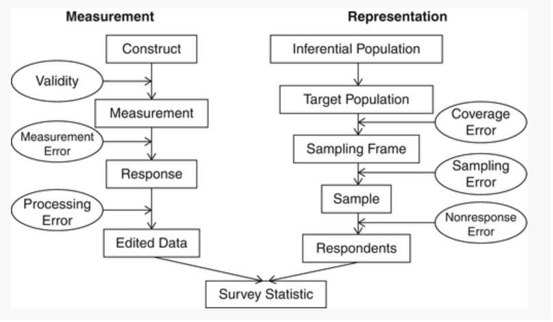
Figure 1.1: Sources of survey errors (Groves et al., 2004)
However, provided they are properly designed and implemented, sample surveys can be (at least) as efficient as censuses, since the size of non-sampling errors is generally smaller when data are collected from a sample of population units than in a census.
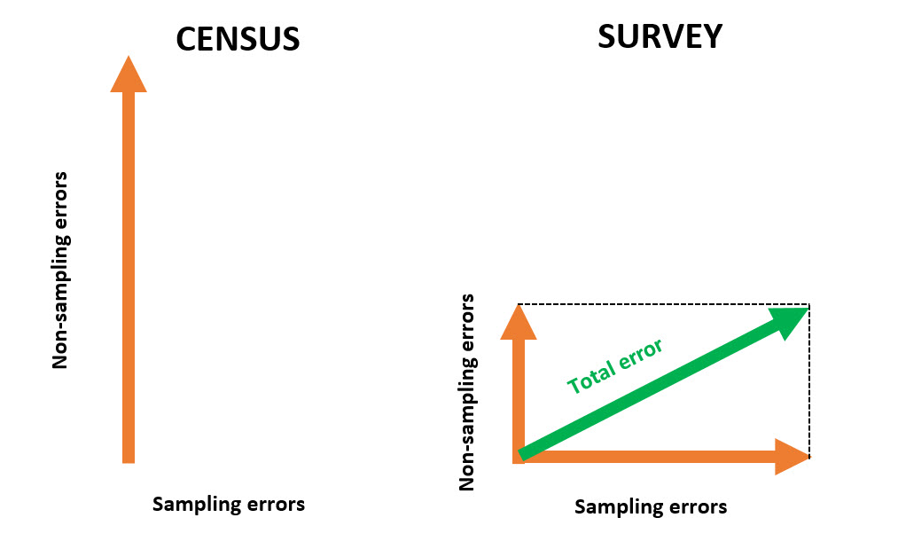
Figure 1.2: Comparison of total error in census and survey data
That’s why, in order to outperform censuses, it is crucial that sample surveys are designed and conducted in such a way that non-sampling errors are as small as possible and that sampling errors are kept under control by having a “large enough” sample. Specifically, considerable resources must be devoted to keeping sampling errors under control; questionnaires must be prepared with the utmost care, subjected to intensive pre-testing and field-testing to detect problems of question wording, routing problems or other inconsistencies; the modes of data collection must be carefully chosen and combined in order to get the most people to cooperate; interviewers must be carefully recruited and properly trained; communication and contact strategies with participants must be designed and adapted to achieve the highest possible participation.
1.4 Main concepts and definitions
1.4.1 Population, sample; parameter and estimator
\(U\) denotes a finite population of \(N\) units. Statistical units must be regarded as a broad concept: physical individuals, households, dwellings, enterprises, agricultural holdings, animals, cars, manufactured goods etc. can be regarded as units from statistical point of view. It is assumed that every unit \(i \in U\) can be completely and uniquely identified by a label. For instance, a natural person can be identified by his first name, surname, gender, date of birth and postal address. A company could be identified by its VAT number or its registration number in a business register.
We seek to estimate a population parameter \(\theta\) which is defined as a function of the \(N\) values of a study variable \(\mathbf{y}\) for each element of the population \(U\):
\[\begin{equation} \theta = \theta\left(\mathbf{y}_i , i \in U\right) \tag{1.1} \end{equation}\]
\(\mathbf{y}_i\) can be either quantitative (e.g. the total disposable income or the total food consumption of a household, profits of an enterprise) or categorical (e.g. distributions by gender, citizenship, country of birth, marital status, occupation or activity status). In the following, \(y\) is supposed to be observed without any error. Therefore \(\left(\mathbf{y}_i , i \in U\right)\) are fixed, non-random values.
\(\theta\) can be a linear parameter of \(\mathbf{y}\), such as a mean \(\bar{Y}=\sum_{i \in U} y_i / N\), a total \(Y=\sum_{i \in U} y_i\) or a proportion; a more complex parameter such as a ratio between two population means, a correlation or a regression coefficient, a quantile (e.g. median, quartile, quintile or decile) or an inequality measure such as the Gini or the Theil indexes:
\[\begin{equation} \theta = \displaystyle{\frac{1}{N}\sum_{i \in U}\frac{y_i}{\bar{Y}} \times \ln \left(\frac{y_i}{\bar{Y}}\right)} \mbox{ (Theil index)} \tag{1.2} \end{equation}\]
In a survey setting, a sample \(s\) of \(n\) units \(\left(n \leq N\right)\) is taken from the population \(U\). In the next chapters, we assume the sample is selected according to a probabilistic design, which means that every element in the population has a fixed known in advance probability to be selected: the probability \(\pi_i\) for a unit \(i \in U\) to be sampled is called the inclusion probability. Otherwise, when the inclusion probabilities are unknown, then the design is said to be empirical or nonprobability. This is what happens for instance in quota sampling, whereby units are selected so to reflect known structures for the population; in expert sampling, whereby sample units are designated from expert advice; or in network sampling, whereby the existing sample units recruit future units from among their ‘network’.
When sample units are selected through a probabilistic design, the sample \(s\) can be regarded as the realization of a random variable \(S\). In most cases, \(s\) is a subset without repetitions of the population (sampling without replacement), although a sample can also be taken with replacement.
Sample observations are used to construct an estimator of the parameter \(\theta\), that is a function of sample observations:
\[\begin{equation} \hat\theta = \hat\theta\left(S\right) = \hat\theta\left(\mathbf{y}_i , i \in S\right) \tag{1.3} \end{equation}\]
For instance, the population mean of the study variable can be estimated by the mean value over the sample observations (see next chapter):
\[\begin{equation} \hat\theta = \frac{\sum_{i \in S} \mathbf{y}_i}{\#S} = \bar{\mathbf{y}}_S \tag{1.4} \end{equation}\]
The size of the selected sample is another example of estimator:
\[\begin{equation} n_S = \sum_{i \in S} 1 \tag{1.5} \end{equation}\]
When \(n_S = n\) then the design is of fixed size.
In survey sampling theory, as the study variable is assumed to be error-free, the random part of an estimator is caused by the probabilistic selection of a sample. This is a major difference in comparison to traditional statistical theory, where the study variable is assumed to follow a given probability distribution (e.g. a normal distribution of mean \(m\) and standard error \(\sigma\)). In survey sampling, statistical inference is design-based that is, with respect to the sampling distribution, while inference in traditional inferential statistics is model-based that is, with respect to the probability distribution of a random variable.
1.4.2 Sampling frame
The actual selection of a sample in a population requires the availability of a sampling frame, i.e. an exhaustive list of all individuals who compose the target population. Luxembourg, for example, has a national population register8 which aims to cover the entire resident population, irrespective of age, nationality or housing conditions. This register is regularly used by STATEC to draw samples for its household surveys. Similarly, Luxembourg has a business register which is used as a sampling frame for business surveys.
In practice, sampling frames are never error-free and cannot cover the target population of a survey exactly. On the one hand, because it takes time to administratively register a person in a register, there will always be some people in the population who are not included in the corresponding sampling frame; on the other hand, a sampling frame also includes people who are no longer eligible (e.g. people who have left the country and may still be included in the register several months after they have left). Discrepancies between the (theoretical) target population of a survey and the frame used to draw a sample are equivalent to statistical errors, called coverage or frame errors.
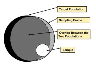
Figure 1.3: Coverage errors
1.4.3 Bias, Variance, Standard error and Mean Square Error
Under probabilistic sampling, several synthetic measures are available in order to assess the statistical quality of an estimator \(\hat\theta\). All these measures are equivalent to those developed in traditional statistical theory:
- Expectation
This is the average value of \(\hat\theta\) over all the possible samples \(\mathcal{S}\) that can be taken from the population:
\[\begin{equation} E\left(\hat\theta\right) = \sum_{s \in \mathcal{S}}Pr\left(S=s\right)\hat\theta\left(S=s\right) \tag{1.6} \end{equation}\]
- Bias
The bias of the estimator \(\hat\theta\) is given by:
\[\begin{equation} B\left(\hat\theta\right) = E\left(\hat\theta\right) - \theta \tag{1.7} \end{equation}\]
If \(B\left(\hat\theta\right)=0\), the estimator \(\hat\theta\) is said to be unbiased. Bias is not measurable as the true value \(\theta\) of the parameter is unknown.
- Variance
The variance of the estimator \(\hat\theta\) is given by:
\[\begin{equation} V\left(\hat\theta\right) = E\left[\hat\theta - E\left(\hat\theta\right)\right]^2 = E\left(\hat\theta^2\right) - E^2\left(\hat\theta\right) \tag{1.8} \end{equation}\]
By taking the square root of the variance, we obtain the standard error:
\[\begin{equation} \sigma\left(\hat\theta\right) = \sqrt{V\left(\hat\theta\right)} \tag{1.9} \end{equation}\]
When the standard error is expressed as a percentage of the parameter \(\theta\), we got the relative standard error or coefficient of variation:
\[\begin{equation} CV\left(\hat\theta\right) = \frac{\sqrt{V\left(\hat\theta\right)}}{\theta} \tag{1.10} \end{equation}\]
- Mean Square Error
The mean square error is a synthetic quality measure summarising bias and variance:
\[\begin{equation} MSE\left(\hat\theta\right) = E\left(\hat\theta - \theta\right)^2 = V\left(\hat\theta\right) + B^2\left(\hat\theta\right) \tag{1.11} \end{equation}\]
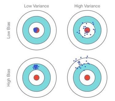
Figure 1.4: Comparison Bias/Variance
The quality of a statistical estimator is seen as a trade-off between bias and variance. In general, bias is often seen as a major problem and we try to keep it as low as possible. Variance is also an issue, but we’ll see that it is directly related to sample size: the larger the sample, the lower the variance. So variance can be kept under control as long as the sample is large enough. Bias, on the other hand, is more difficult to deal with because it is related to other design factors such as the questionnaire or the way the data is collected.
Numerical example: Consider a population of \(N\)=5 elements, labelled \(i = 1 \cdots 5\), and a study variable \(y_i\) for each population elements. \[\begin{equation} \begin{array}{|c|c|} i & \textbf{y} \\ 1 & 2 \\ 2 & 5 \\ 3 & 8 \\ 4 & 4 \\ 5 & 1 \\ \end{array} \end{equation}\]
Consider a sampling design in which every sample of size 2 has the same probability, equal to 1/10, to be selected. The probability is zero when the sample size is different from 2.
We seek to estimate the population mean of the study variable \(y\) that is, \(\bar{Y} = \displaystyle{\frac{y_1 + y_2 + y_3 + y_4 + y_5}{5}} = 4\).
To that end, we use the sample mean \(\bar{y}\) as an estimator of \(\bar{Y}\). We got the following: \[\begin{equation} \begin{array}{|c|c|c|} s & Pr\left(S=s\right) & \bar{y} \\ \{1,2\} & 0.1 & 3.5 \\ \{1,3\} & 0.1 & 5.0 \\ \{1,4\} & 0.1 & 3.0 \\ \{1,5\} & 0.1 & 1.5 \\ \{2,3\} & 0.1 & 6.5 \\ \{2,4\} & 0.1 & 4.5 \\ \{2,5\} & 0.1 & 3.0 \\ \{3,4\} & 0.1 & 6.0 \\ \{3,5\} & 0.1 & 4.5 \\ \{4,5\} & 0.1 & 2.5 \\ \end{array} \end{equation}\]
The bias of the sample mean is given by: \[0.1 \left(3.5 + 5.0 + 3.0 + 1.5 + 6.5 + 4.5 + 3.0 + 6.0 + 4.5 + 2.5\right) = 4 = \bar{Y}\]
Therefore the estimator is unbiased. As regards the variance, we have: \[\begin{equation} \begin{array}{|c|c|c|} s & Pr\left(S=s\right) & \left(\bar{y}-\bar{Y}\right)^2 \\ \{1,2\} & 0.1 & 0.5^2 \\ \{1,3\} & 0.1 & 1.0^2 \\ \{1,4\} & 0.1 & 1.0^2 \\ \{1,5\} & 0.1 & 2.5^2 \\ \{2,3\} & 0.1 & 2.5^2 \\ \{2,4\} & 0.1 & 0.5^2 \\ \{2,5\} & 0.1 & 1.0^2 \\ \{3,4\} & 0.1 & 2.0^2 \\ \{3,5\} & 0.1 & 0.5^2 \\ \{4,5\} & 0.1 & 1.5^2 \\ \end{array} \end{equation}\]
The variance of the sample mean is given by: \(0.1 \left(0.25 + 1.0 + 1.0 + 6.25 + 6.25 + 0.25 + 1.0 + 4.0 + 0.25 + 2.25\right) = 2.25\)
Hence, the standard error is given by \(\sqrt{2.25}=1.5\) and the relative standard error is \(1.5 / 4 = 37.5\%\)
1.4.4 Confidence interval
Finally, the estimated standard error is used to determine a confidence interval within which the target parameter \(\theta\) lies with a very high probability, close to 1. The statistical process of extrapolating results from sample observations to the entire survey population (in the form of a confidence interval) is called statistical inference.
Assuming the estimator \(\hat\theta\) is both unbiased and normally distributed, a confidence interval for \(\theta\) at level \(1 - \alpha\) is given by:
\[\begin{equation} CI\left(\theta\right) = \left[\hat\theta - q_{1-\alpha/2}\times \sigma\left(\hat\theta\right) ~,~ \hat\theta + q_{1-\alpha/2}\times\sigma\left(\hat\theta\right)\right] \tag{1.12} \end{equation}\]
where \(q_{1-\alpha/2}\) is the quantile at \(1-\alpha/2\) of the normal distribution of mean 0 and standard error 1. For example, we have:
- \(\alpha = 0.1 \Rightarrow q_{1-\alpha/2}=1.65\)
- \(\alpha = 0.05 \Rightarrow q_{1-\alpha/2}=1.96\)
- \(\alpha = 0.01 \Rightarrow q_{1-\alpha/2}=2.58\)
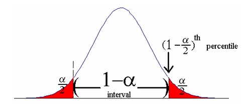
Figure 1.5: Confidence interval
The quantity \(q_{1-\alpha/2} \times \sigma\left(\hat\theta\right)\) that is, the half-length of the confidence interval, is the (absolute) margin of error. When the latter is expressed as a percentage of the population parameter \(\theta\), we obtain the relative margin of error of \(\hat\theta\).
In practice the standard error \(\sigma\left(\hat\theta\right)\) is unknown and is estimated by \(\hat\sigma\left(\hat\theta\right)\). Thus, we obtain the following estimated confidence interval through substituting \(\hat\sigma\left(\hat\theta\right)\) for \(\sigma\left(\hat\theta\right)\):
\[\begin{equation} \hat{CI}\left(\theta\right) = \left[\hat\theta - q_{1-\alpha/2}\times \hat\sigma\left(\hat\theta\right) ~,~ \hat\theta + q_{1-\alpha/2}\times \hat\sigma\left(\hat\theta\right)\right] \tag{1.13} \end{equation}\]
The normality assumption underlying (1.12) is generally valid provided the sample size is large enough. If the sample size is too small, the quantile \(q_{1-\alpha/2}\) of the normal distribution can be replaced by the quantile of the t-distribution (Student) with degrees of freedom \(n-1\). Regarding the unbiasedness of the estimator \(\hat\theta\), this property can be verified under ideal conditions (e.g. simple random sampling). However, it is not satisfied under general survey conditions, mainly because of the negative effect of non-sampling errors. In this case, the bias leads to a distortion of the confidence level in the sense that the theoretical value \(1 - \alpha\) is actually higher than the real value when the bias ratio \(B\left(\hat\theta\right) / \sigma\left(\hat\theta\right)\) is too high:

A major advantage of calculating confidence intervals is that they are easy to understand and interpret, unlike the more complex measures of variance and standard error. The latter two measures are not the ultimate goal in statistical inference, but rather an intermediate step in the construction of valid confidence intervals.
https://www.ecb.europa.eu/stats/ecb_surveys/html/index.en.html↩︎
Registre National des Personnes Physiques (RNPP)↩︎