Chapter 5 Multistage sampling
5.1 Introduction and notations
The sampling designs presented so far are single-stage designs that is, sampling frames are available for direct-element selection. However, there exists many practical situations where no frame is available in order to identify the elements of a population. In which case, multi-stage sampling is an alternative option:
- At first-stage sampling, a sample of Primary Sampling Units (PSU) is selected using a probabilistic design (e.g. simple random sampling or other, with or without stratification)
- At second-stage sampling, a sub-sample of Secondary Sampling Units (SSU) is selected within each PSU selected at first-stage. The selection of SSU is supposed to be independent from one PSU to another.
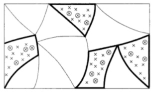
Figure 5.1: Principle of multistage sampling (Ardilly, 2006)
The process can be continued and at third-stage sampling a sample of Tertiary Sampling Units can be selected with each of the SSU selected at second stage.
For example, in the absence of any frame of individuals, we may consider selecting a sample of municipalities (first-stage sampling), a sample of neighbourhoods (second-stage sampling) within each selected municipality, a sample of households (third-stage sampling) within each of the neighbourhoods selected a second stage and finally a sample of individuals (fourth-stage sampling) within each household.
5.2 Estimating a population total
We wish to estimate the total \(Y\) of a study variable \(y\): \[ Y = \sum_{i \in U_I} \sum_{j \in U_{IIi}} y_{ij} = \sum_{i \in U_I} Y_{i} \] where
- \(y_{ij}\) is the value taken by \(y\) on the SSU \(j\) of PSU \(i\)
- \(Y_i = \sum_{j \in U_{IIi}} y_{ij}\) is the subtotal of \(y\) on PSU \(i\)
According to the Horvitz-Thompson principle, \(Y\) should be estimated by the following sum: \(\sum_{i \in s_I} Y_{i} / \pi_{Ii}\), where \(\pi_{Ii}\) is the inclusion probability of PSU \(i\).
As the term \(Y_i\) is unknown, it must be estimated using the same Horvitz-Thompson principle. As a result, in two-stage sampling, the total \(Y\) of \(y\) is estimated by the following two-stage Horvitz-Thompson estimator:
\[\begin{equation} \begin{array}{rcl} \hat{Y}_{HT,2st} & = & \displaystyle{\sum_{i \in s_I} \frac{\hat{Y}_{i,HT}}{\pi_{Ii}}} \\ & = & \displaystyle{\sum_{i \in s_I} \sum_{j \in s_{IIi}} \frac{y_{ij}}{\pi_{Ii} \pi_{IIj}}} \end{array} \tag{5.1} \end{equation}\]
where \(\pi_{IIj}\) is the conditional inclusion probability of SSU \(j\) given PSU \(i\) had been selected at first-stage.
The variance of \(\hat{Y}_{HT,2st}\) is given by:
\[\begin{equation} \begin{array}{rcl} V\left(\hat{Y}_{HT,2st}\right) & = & \displaystyle{\sum_{i \in U_I}\sum_{i' \in U_I} \Delta_{Iii'}\frac{Y_i}{\pi_{Ii}}\frac{Y_{i'}}{\pi_{Ii'}} + \sum_{i \in U_I} \frac{V\left(\hat{Y}_{i,HT}\right)}{\pi_{Ii}}} \end{array} \tag{5.2} \end{equation}\]
where
- \(V_I = \displaystyle{\sum_{i \in U_I}\sum_{i' \in U_I}\Delta_{Iii'}\frac{Y_i}{\pi_{Ii}}\frac{Y_{i'}}{\pi_{Ii'}}}\) is the first-stage variance
- \(V_{II} = \displaystyle{\sum_{i \in U_I} \frac{V\left(\hat{Y}_{i,HT}\right)}{\pi_{Ii}}}\) is the second-stage variance
Proof: the variance is decomposed into first-stage variance and second-stage variance using conditional expectation and conditional variance
\[\begin{equation} \begin{array}{ccc} V\left(\hat{Y}_{HT,2st}\right) & = & V_I\left[E_{II}\left(\hat{Y}_{HT,2st} | I\right)\right] + E_I\left[V_{II}\left(\hat{Y}_{HT,2st} | I\right)\right] \\ & = & \displaystyle{V_I\left(\sum_{i \in s_I} \frac{{Y}_{i}}{\pi_{Ii}}\right) + E_I\left[\sum_{i \in s_I} \frac{V\left(\hat{Y}_{i,HT}\right)}{\pi^2_{Ii}}\right]} \\ & = & \displaystyle{\sum_{i \in U_I}\sum_{i' \in U_I}\Delta_{Iii'}\frac{Y_i}{\pi_{Ii}}\frac{Y_{i'}}{\pi_{Ii'}} + \sum_{i \in U_I} \frac{V\left(\hat{Y}_{i,HT}\right)}{\pi_{Ii}}} \end{array} \end{equation}\]
The variance (5.2) is unbiasedly estimated by:
\[\begin{equation} \begin{array}{rcl} \hat{V}\left(\hat{Y}_{HT,2st}\right) & = & \displaystyle{\sum_{i \in s_I}\sum_{i' \in s_I} \frac{\Delta_{Iii'}}{\pi_{Iii'}}\frac{\hat{Y}_{i,HT}}{\pi_{Ii}}\frac{\hat{Y}_{i',HT}}{\pi_{Ii'}} + \sum_{i \in s_I} \frac{\hat{V}\left(\hat{Y}_{i,HT}\right)}{\pi_{Ii}}} \end{array} \tag{5.3} \end{equation}\]
where \(\hat{V}\left(\hat{Y}_{i,HT}\right)\) is an unbiased estimator of the variance \({V}\left(\hat{Y}_{i,HT}\right)\)
Proof: \[\begin{equation} \begin{array}{rcl} & & \displaystyle{E_{II}\left(\sum_{i \in s_I}\sum_{i' \in s_I} \frac{\Delta_{Iii'}}{\pi_{Iii'}}\frac{\hat{Y}_{i,HT}}{\pi_{Ii}}\frac{\hat{Y}_{i',HT}}{\pi_{Ii'}}|I\right)} \\ & = & \displaystyle{\sum_{i \in s_I}\sum_{\substack {i' \in s_I \\ i' \neq i}} \frac{\Delta_{Iii'}}{\pi_{Iii'}}\frac{E_{II}\left({\hat{Y}}_{i,HT}{\hat{Y}}_{i',HT}|I\right)}{\pi_{Ii}\pi_{Ii'}} + \sum_{i \in s_I} \frac{\Delta_{Ii}}{\pi_{Ii}}\frac{E_{II}\left(\hat{Y}^2_{i,HT}|I\right)}{\pi^2_{Ii}}} \\ & = & \displaystyle{\sum_{i \in s_I}\sum_{\substack {i' \in s_I \\ i' \neq i}} \frac{\Delta_{Iii'}}{\pi_{Iii'}}\frac{E_{II}\left({\hat{Y}}_{i,HT}|I\right)E_{II}\left({\hat{Y}}_{i',HT}|I\right)}{\pi_{Ii}\pi_{Ii'}} + \sum_{i \in s_I} \frac{\Delta_{Ii}}{\pi_{Ii}}\frac{E^2_{II}\left(\hat{Y}_{i,HT}|I\right) + V\left(\hat{Y}_{i,HT}\right)}{\pi^2_{Ii}}}\\ & = & \displaystyle{\sum_{i \in s_I}\sum_{i' \in s_I} \frac{\Delta_{Iii'}}{\pi_{Iii'}}\frac{E_{II}\left({\hat{Y}}_{i,HT}|I\right)E_{II}\left({\hat{Y}}_{i',HT}|I\right)}{\pi_{Ii}\pi_{Ii'}} + \sum_{i \in s_I} \frac{\Delta_{Ii}}{\pi_{Ii}}\frac{V\left(\hat{Y}_{i,HT}\right)}{\pi^2_{Ii}}} \\ & = & \displaystyle{\sum_{i \in s_I}\sum_{i' \in s_I} \frac{\Delta_{Iii'}}{\pi_{Iii'}}\frac{{Y}_{i} {Y}_{i'}}{\pi_{Ii}\pi_{Ii'}} + \sum_{i \in s_I} \frac{1-\pi_{Ii}}{\pi^2_{Ii}}{V\left(\hat{Y}_{i,HT}\right)}} \end{array} \end{equation}\]
Thus we got \[\begin{equation} \begin{array}{rcl} & & \displaystyle{E\left(\sum_{i \in s_I}\sum_{i' \in s_I} \frac{\Delta_{Iii'}}{\pi_{Iii'}}\frac{\hat{Y}_{i,HT}}{\pi_{Ii}}\frac{\hat{Y}_{i',HT}}{\pi_{Ii'}}\right)} \\ & = & \displaystyle{\sum_{i \in U_I}\sum_{i' \in U_I} \Delta_{Iii'}\frac{Y_i}{\pi_{Ii}}\frac{Y_{i'}}{\pi_{Ii'}} + \sum_{i \in U_I} \frac{1-\pi_{Ii}}{\pi_{Ii}}{V\left(\hat{Y}_{i,HT}\right)}} \\ & = & \displaystyle{\sum_{i \in U_I}\sum_{i' \in U_I} \Delta_{Iii'}\frac{Y_i}{\pi_{Ii}}\frac{Y_{i'}}{\pi_{Ii'}} + \sum_{i \in U_I} \frac{V\left(\hat{Y}_{i,HT}\right)}{\pi_{Ii}} - \sum_{i \in U_I} V\left(\hat{Y}_{i,HT}\right)} \\ & = & \displaystyle{V\left(\hat{Y}_{HT,2st}\right) - \sum_{i \in U_I} V\left(\hat{Y}_{i,HT}\right)} \end{array} \end{equation}\]
As we have:
\[\begin{equation} \displaystyle{E\left(\sum_{i \in s_I} \frac{\hat{V}\left(\hat{Y}_{i,HT}\right)}{\pi_{Ii}}\right) = \sum_{i \in U_I} {V}\left(\hat{Y}_{i,HT}\right)} \end{equation}\]
then we can conclude (5.3) is an unbiased estimator of the variance.
The first term of (5.3) (“Ultimate Cluster” estimator) is often considered as a more tractable option for variance estimation under multi-stage sampling, though this estimator is slightly biased.
\[\begin{equation} \begin{array}{rcl} \hat{V}_{UC}\left(\hat{Y}_{HT,2st}\right) & = & \displaystyle{\sum_{i \in s_I}\sum_{i' \in s_I} \frac{\Delta_{Iii'}}{\pi_{Iii'}}\frac{\hat{Y}_{i,HT}}{\pi_{Ii}}\frac{\hat{Y}_{i',HT}}{\pi_{Ii'}}} \end{array} \tag{5.4} \end{equation}\]
However the bias should be negligible as long as the first-stage inclusion probabilities \(\pi_{Ii}\) are small. In which case, assuming sampling with replacement, the Hansen-Hurwitz estimator can be used as a sensible estimator for the variance under multi-stage sampling:
\[\begin{equation} \begin{array}{rcl} \hat{V}_{UC}\left(\hat{Y}_{HT,2st}\right) & = & \displaystyle{\frac{1}{m}\frac{1}{m-1}\sum_{i \in s_I}\left(\frac{\hat{Y}_{i,HT}}{p_{Ii}}-\hat{Y}_{HT,2st}\right)^2} \end{array} \tag{5.5} \end{equation}\]
where \(m\) is the number of PSUs drawn at first stage and \(p_{Ii} = \pi_{Ii} / m\).
(5.5) is general enough to accommodate most of the multi-stage sampling designs used in practice. The formula works under mild assumptions, mainly the sampling fraction at first stage be close to zero.
If not, the variance formula (5.5) can be adjusted using the finite population correction factor at first stage:
\[\begin{equation} \begin{array}{rcl} \hat{V}_{UC}\left(\hat{Y}_{HT,2st}\right) & = & \displaystyle{\left(1-f\right)\frac{1}{m}\frac{1}{m-1}\sum_{i \in s_I}\left(\frac{\hat{Y}_{i,HT}}{p_{Ii}}-\hat{Y}_{HT,2st}\right)^2} \end{array} \tag{5.6} \end{equation}\]
where \(1-f = 1-\displaystyle{\frac{m}{M}}\)
5.3 Case of simple random sampling at each stage
Let assume simple random sampling of \(m\) PSUs out of \(M\) at first stage and, within each PSU \(i\), simple random sampling of \(n_i\) SSUs out of \(N_i\). Then the variance (5.2) can be written as:
\[\begin{equation} \begin{array}{rcl} V\left(\hat{Y}_{HT,2st}\right) & = & \displaystyle{M^2 \left(1-\frac{m}{M}\right) \frac{S_Y^2}{m} + \frac{M}{m}\left[\sum_{i \in U_{I}} N^2_i \left(1-\frac{n_i}{N_i}\right)\frac{S^2_i}{n_i}\right]} \end{array} \tag{5.7} \end{equation}\]
where: \(S_Y^2\) is the dispersion among the PSU totals \(Y_i\)
When we assume \(n_i=N_i ~~\forall i\) (cluster sampling) and \(N_i=\bar{N} ~~\forall i\), the variance (5.7) can be written as:
\[\begin{equation} \begin{array}{rcl} V\left(\hat{Y}_{HT,2st}\right) & = & \displaystyle{M^2 \left(1-\frac{m}{M}\right) \frac{S_Y^2}{m}} \\ & \approx & \displaystyle{N^2 \left(1-\frac{n}{N}\right) \frac{S^2}{n} \left[1 + \rho\left(\bar{N}-1\right)\right]} \end{array} \tag{5.8} \end{equation}\]
where \(\rho\) denotes the intra-cluster correlation coefficient: the more homogeneous the PSU with regard to the characteristics of interest, the higher the coefficient.
\[\begin{equation} \displaystyle{\rho = \frac{1}{\bar{N}-1}\frac{\sum_{i \in U_I} \sum_{j \in U_{IIi}} \sum_{\substack {k \in U_{IIi} \\ k \neq j}} \left(y_{ij} - \bar{Y}\right) \left(y_{ik} - \bar{Y}\right)}{\sum_{i \in U_I} \sum_{j \in U_{IIi}} \left(y_{ij} - \bar{Y}\right)^2} \approx \frac{S^2_B}{S^2}-\frac{1}{\bar{N}}} \tag{5.9} \end{equation}\]
The factor \(\left[1 + \rho\left(\bar{N}-1\right)\right]\) measures the gain or loss in accuracy due to clustering as compared to simple random sampling of same size. This coefficient is known as the design effect factor (Deff). If \(\rho > 0\) then clustering leads to a loss in accuracy as compared to simple random sampling, while \(\rho < 0\) means that clustering has had a postive effect on sample accuracy.
In short, in order to reduce the negative impact of clustering on accuracy, PSU should be constructed so to be as heterogeneous as possible with respect to the target characteristics of the study, and to be as small as possible. This is a logic which is different to that of stratification, where strata must be as homogeneous as possible in order to be efficient in term of variance reduction. Actually, stratification can be combined with multistage selection in order to offset the loss of accuracy due to clustering.
5.4 Design optimality
The result (5.8) can be extended beyond cluster sampling to two-stage sample selection where the sample size \(\bar{n}\) at second stage is equal within each PSU. In which case, the variance is:
\[\begin{equation} V\left(\hat{Y}_{HT,2st}\right) \approx \displaystyle{N^2 \frac{S^2}{n} \left[1 + \rho\left(\bar{n}-1\right)\right]} = \displaystyle{N^2 S^2 \left[ \frac{1-\rho}{m\bar{n}} + \frac{\rho}{m}\right]} \tag{5.10} \end{equation}\]
Ther above formula can be used to determine the optimal sample sizes \(m\) and \(\bar{n}\) at each sampling stage so to minimise the variance (5.10) under the cost constraint \(c_1m+c_2m\bar{n}=C\). We got the following result:
\[\begin{equation} \begin{array}{rcl} \bar{n}& = & \displaystyle{\sqrt{\frac{c_1}{c_2}\frac{1-\rho}{\rho}}} \\ m & = & \displaystyle{\frac{C}{c_1 + \sqrt{c_1 c_2 \displaystyle{\frac{1-\rho}{\rho}}}}} \end{array} \tag{5.11} \end{equation}\]
Therefore, when the average cost \(c_1\) of surveying a PSU is low compared to the cost \(c_2\) for a SSU, then we have to put the effort on sample size \(m\) at first stage in order to reach optimal accuracy under cost constraints.