Chapter 24 Model Building
Author: Ron Reviewer:
24.1 Introduction
24.1.1 prerequisites
library(tidyverse)
library(modelr)
options(na.action = na.warn)

library(nycflights13)
library(lubridate)
24.2 Why are low quality diamonds more expensive
24.2.1 Price and carat
Note:
Residuals of a model contain the information that doesn’t get caught by this model. By examining the residual of the following model
fit1 <- lm(data = diamonds,log(price)~log(carat))A positive relationship of the residual with one additional predictor means there is a positive correlation between them. For example, residual ~ cut means cut may partially explain the increase of the prediction error of fit1. This becomes more obvious when the residual is transformed back from log scale which explains the exponential price growth with respect to cut or clarity.
24.2.2 A more complicated model
24.2.3 Exercises
1.In the plot of lcarat vs. lprice, there are some bright vertical strips. What do they represent?
diamonds2 <- diamonds %>%
  filter(carat <= 2.5) %>%
  mutate(lprice = log2(price), lcarat = log2(carat))

ggplot(diamonds2, aes(lcarat, lprice)) +
  geom_hex(bins = 50)
## Warning: Computation failed in `stat_binhex()`:
## Package `hexbin` required for `stat_binhex`.
## Please install and try again.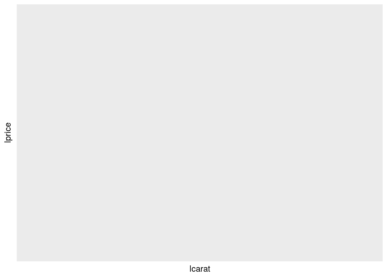 Those bright vertical strips mean that many diamonds are cut to those “standard” or popular “weight” since bright means higher count.
2.If log(price) = a_0 + a_1 * log(carat), what does that say about the relationship between price and carat?
It means price = exp(a_0)*carat^(a_1).
3.Extract the diamonds that have very high and very low residuals. Is there anything unusual about these diamonds? Are the particularly bad or good, or do you think these are pricing errors?
diamonds2 <- diamonds %>%
  filter(carat <= 2.5) %>%
  mutate(lprice = log2(price), lcarat = log2(carat))

mod_diamond <- lm(lprice ~ lcarat, data = diamonds2)

diamonds2 <- diamonds2 %>%
  add_residuals(mod_diamond,'lresid')

summary(diamonds2$lresid)
## Min. 1st Qu. Median Mean 3rd Qu. Max.
## -1.964068 -0.245488 -0.008442 0.000000 0.239301 1.934855diamonds3 <- diamonds2 %>% filter(lresid > quantile(lresid)[[3]] | lresid < quantile(lresid)[[1]] )
table(diamonds3$cut)##
## Fair Good Very Good Premium Ideal
## 317 1651 5515 6477 12946table(diamonds3$clarity)##
## I1 SI2 SI1 VS2 VS1 VVS2 VVS1 IF
## 1 836 4321 7340 5304 4208 3225 1671diamonds3 %>%
ggplot(aes(clarity,price))+
geom_boxplot()+
facet_grid(~cut)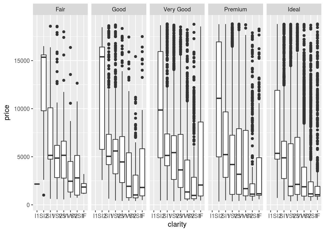 There are surely errrs here. diamonds with better clarity are priced lower.
- No. Since the predictors are not normalized and treated equally in the model. There are some diamonds which are very expensive but predicted to be cheap or vice versa.
24.3 What affects the number of daily flights
24.3.1 Day of week
Some useful functions from package lubridate
# make date
lubridate::make_date(1992,8,12)
## [1] "1992-08-12"# find weekday
lubridate::make_date(1992,8,12) %>%
lubridate::wday(label = TRUE)## [1] Wed
## Levels: Sun < Mon < Tue < Wed < Thu < Fri < Sat# make date as year month day
lubridate::ymd(20130101)## [1] "2013-01-01"24.3.2 Seasonal Saturday effect
daily <- flights %>%
  mutate(date = make_date(year, month, day)) %>%
  group_by(date) %>%
  summarise(n = n())
daily <- daily %>%
  mutate(wday = wday(date, label = TRUE))
daily %>%
filter(wday == "Sat") %>%
ggplot(aes(date, n)) +
geom_point() +
geom_line() +
scale_x_date(NULL, date_breaks = "1 month", date_labels = "%b") # set x tick as a month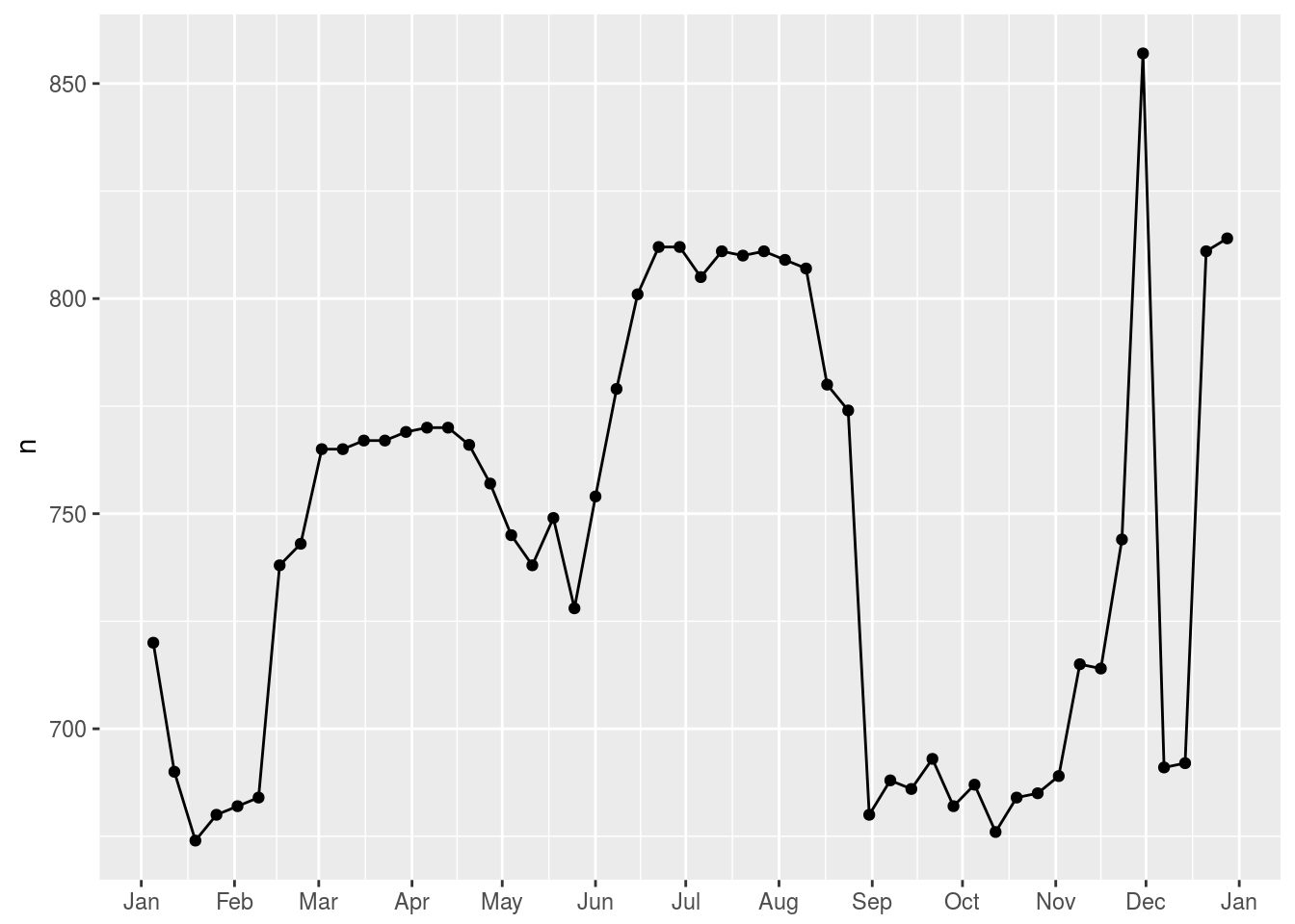
24.3.3 Computed variables
Note:
It is preferred to make computed/transformed variables explicit for further visualization purpose if memory permits.
24.3.4 Time of year: an alternative approach
24.3.5 Exercises
- Use your Google sleuthing skills to brainstorm why there were fewer than expected flights on Jan 20, May 26, and Sep 1. (Hint: they all have the same explanation.) How would these days generalise to another year?
They are close to the Martin Luther King day, the trinity Sunday and the Labor day. They can’t be generalised to other years because those dates depend on weekdays.
Check the website.
- What do the three days with high positive residuals represent? How would these days generalise to another year?
# repeat what is done in the book
term <- function(date) {
  cut(date,
    breaks = ymd(20130101, 20130605, 20130825, 20140101),
    labels = c("spring", "summer", "fall")
  )
}

daily <- daily %>%
  mutate(term = term(date))

daily %>%
  filter(wday == "Sat") %>%
  ggplot(aes(date, n, colour = term)) +
  geom_point(alpha = 1/3) +
  geom_line() +
  scale_x_date(NULL, date_breaks = "1 month", date_labels = "%b")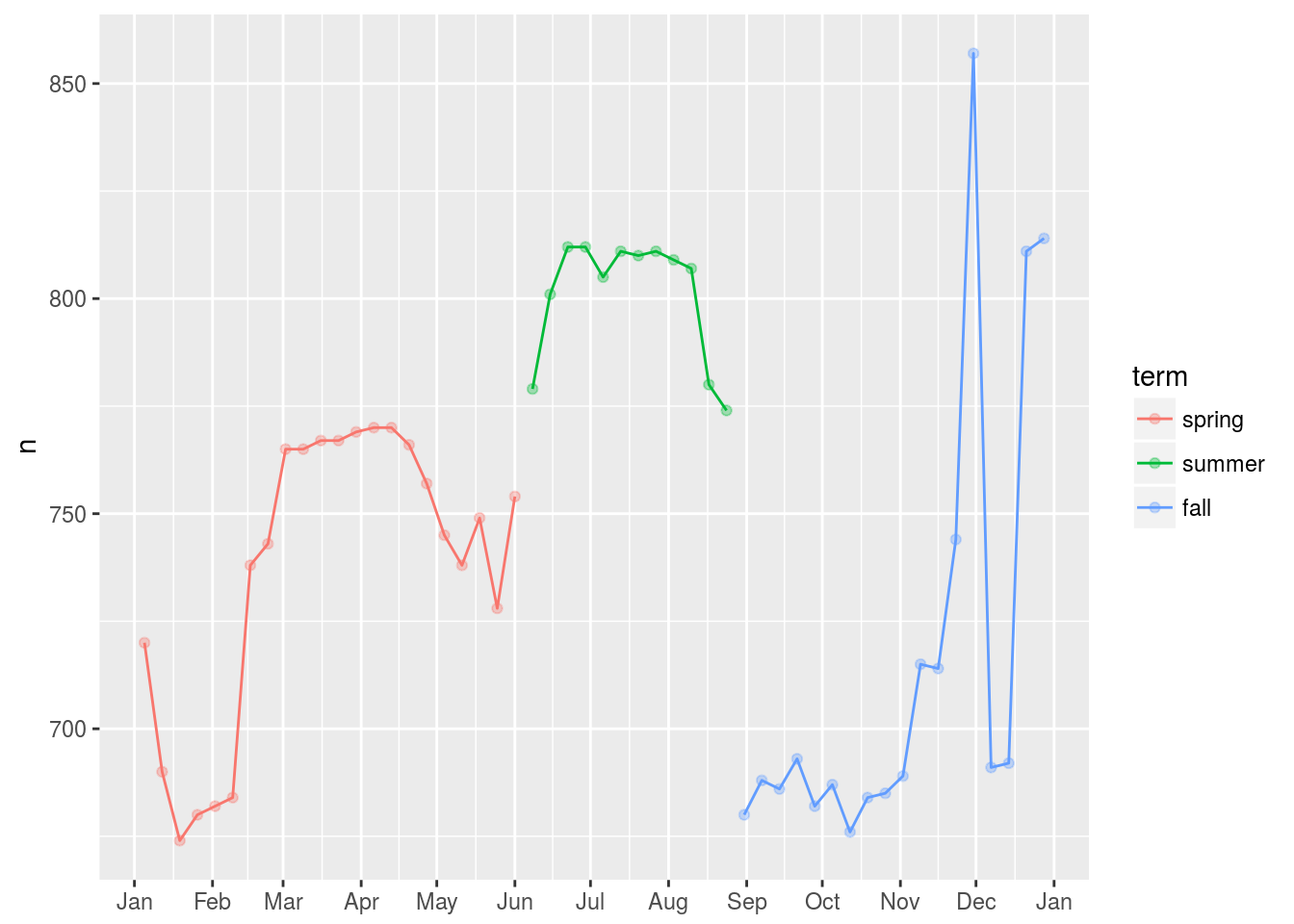
mod1 <- lm(n ~ wday, data = daily)
mod2 <- lm(n ~ wday * term, data = daily)

daily %>%
  gather_residuals(without_term = mod1, with_term = mod2) %>%
  ggplot(aes(date, resid),color = model) +
    geom_line(alpha = 0.75) +
  facet_grid(~model)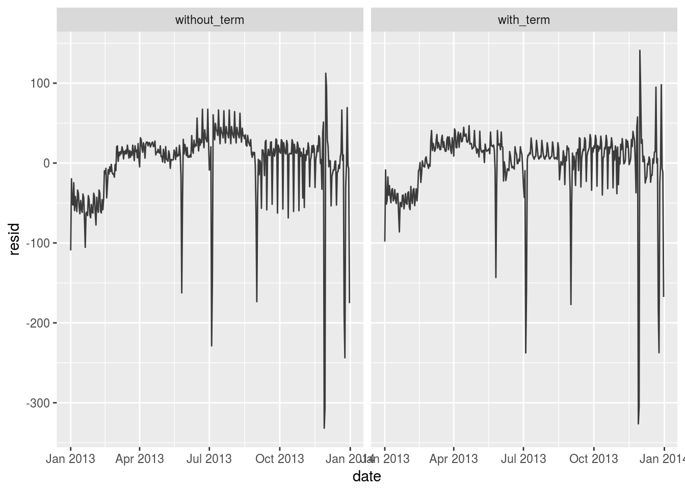
daily %>%
  add_residuals(mod1) %>%
  add_predictions(mod1) %>%
  top_n(3, resid)
## # A tibble: 3 x 6
## date n wday term resid pred
## <date> <int> <ord> <fctr> <dbl> <dbl>
## 1 2013-11-30 857 Sat fall 112.38462 744.6154
## 2 2013-12-01 987 Sun fall 95.51923 891.4808
## 3 2013-12-28 814 Sat fall 69.38462 744.6154Those dates are close to Thanks giving and New Year. The travel need is high.
- Create a new variable that splits the wday variable into terms, but only for Saturdays, i.e. it should have
Thurs,Fri, butSat-summer,Sat-spring,Sat-fall. How does this model compare with the model with every combination ofwdayandterm?
daily <- daily %>%
  mutate(term = term(date))  %>%
  mutate(term2 = ifelse(wday == 'Sat',paste0(wday,"-",term),as.character(term) ))

mod3 <- lm(n~ wday * term2, data = daily)

daily %>%
  gather_residuals(mod3,mod2)%>%
  arrange(date)%>%
  ggplot(aes(date,resid,color = model))+
  geom_line(alpha = 0.75)
## Warning in predict.lm(model, data): prediction from a rank-deficient fit
## may be misleading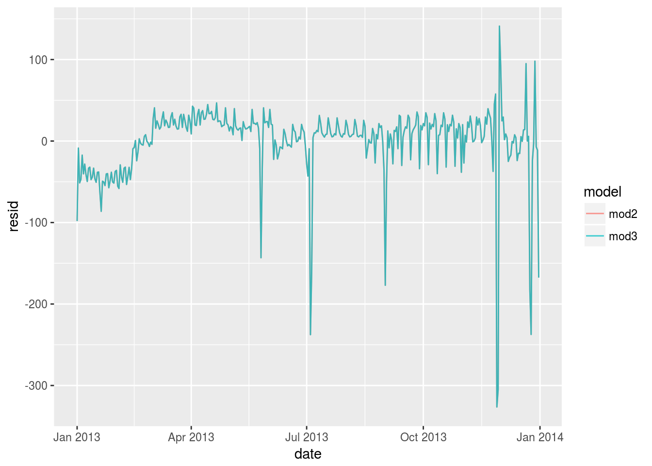 We get a warning saying that
 prediction from a rank-deficient fit may be misleading. This is understandable since our term2 variable is constructed from term and wday. The prediction result is exactly the same.
- Create a new
wdayvariable that combines the day of week, term (for Saturdays), and public holidays. What do the residuals of that model look like? chron package has a function calledis.holidayRequires additonal work to identify American Public holidays
# to do5.What happens if you fit a day of week effect that varies by month (i.e. n ~ wday * month)? Why is this not very helpful?
daily <- flights %>%
mutate(date = make_date(year, month, day)) %>%
group_by(date,month) %>%
summarise(n = n())
daily <- daily %>%
mutate(wday = wday(date, label = TRUE)) %>%
mutate(term = term(date))
mod2 <- lm(n ~ wday * term, data = daily)
mod4 <- lm(n~ wday * month, data = daily)
daily %>%
gather_residuals(mod4,mod2)%>%
arrange(date)%>%
ggplot(aes(date,resid,color = model))+
geom_line(alpha = 0.75)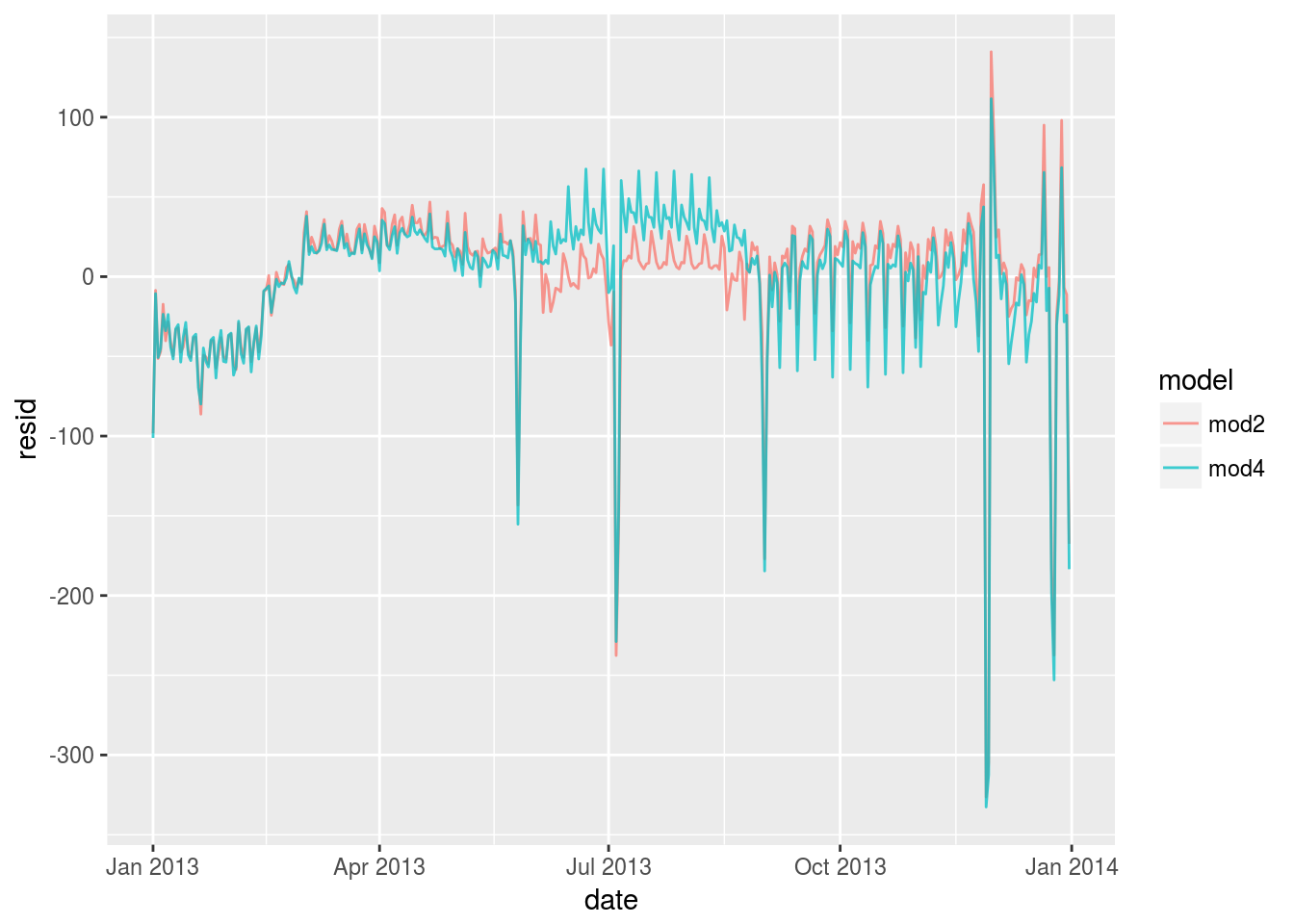 It can be understood this way that
 month information is part of the date information so the performance will be actually a little bit worse.
- What would you expect the model
n ~ wday + ns(date, 5)to look like? Knowing what you know about the data, why would you expect it to be not particularly effective?
mod5 <- lm(n ~ wday + splines::ns(date, 5), data = daily)
daily %>%
  gather_residuals(mod2,mod5)%>%
  arrange(date)%>%
  ggplot(aes(date,resid,color = model))+
  geom_line(alpha = 0.75)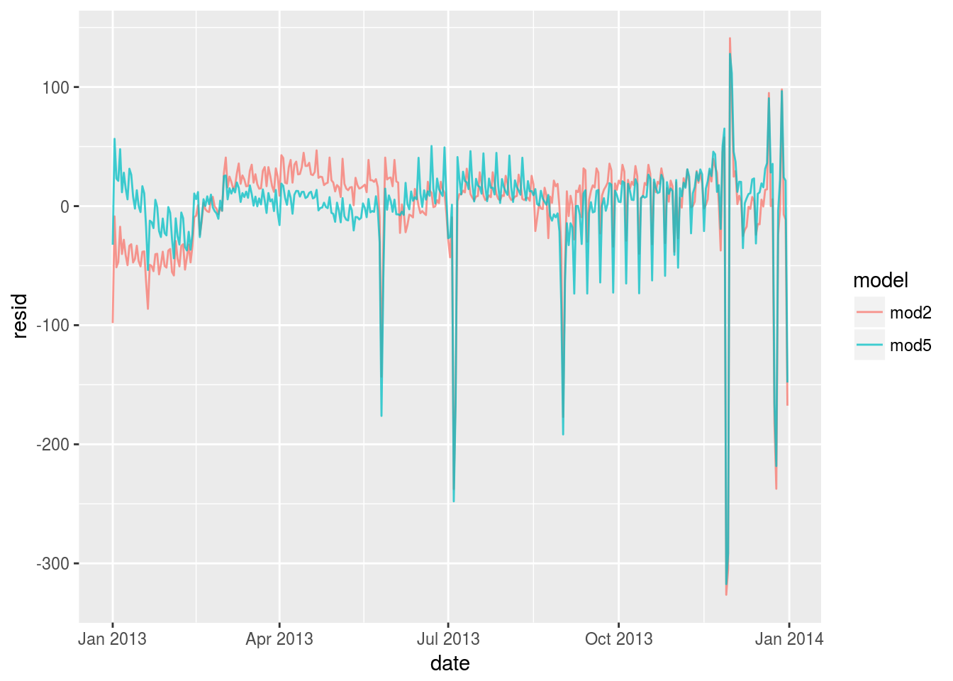
Splines does better job when n changes slowly but it has a systematic overestimation in the fall semester. It shouldn’t be particularly effective.
- We hypothesised that people leaving on Sundays are more likely to be business travellers who need to be somewhere on Monday. Explore that hypothesis by seeing how it breaks down based on distance and time: if it’s true, you’d expect to see more Sunday evening flights to places that are far away.
dist <- function(distance) {
  cut(distance,
    breaks = seq(min(flights$distance,na.rm = TRUE),max(flights$distance,na.rm = TRUE),length.out = 10),
    labels = letters[1:9]
  )
}

time <- function(air_time){
    cut(air_time,
    breaks = seq(min(flights$air_time,na.rm = TRUE),max(flights$air_time,na.rm = TRUE),length.out = 10),
    labels = letters[1:9]
  )
}

dep <- function(dep_time){
    cut(dep_time,
    breaks = seq(0000,2400,length.out = 9),
    labels = c("0-3","3-6","6-9","9-12","12-15","15-18","18-21","21-24")
  )
}

flights <- flights %>%
  mutate(dist = dist(distance)) %>%
  mutate(time = time(air_time)) %>%
  mutate(dep = dep(dep_time))%>%
  mutate(wday= wday(make_date(year, month, day), label = TRUE))
Visualize the flights distance distribution
flights %>%
ggplot() +
geom_bar(aes(dep,color = dist),position = "dodge") +
facet_wrap(~wday, nrow=3)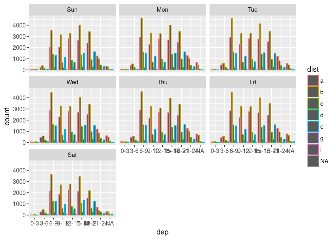 As far as the graph explains, the hypothesis is not true.
8.It’s a little frustrating that Sunday and Saturday are on separate ends of the plot. Write a small function to set the levels of the factor so that the week starts on Monday.
Reorder the factor wday.
flights <- rbind(flights %>% filter(wday != 'Sun'),flights %>% filter(wday == 'Sun'))24.4 Learning more about models
Statistical Modeling: A Fresh ApproachAn Introduction to Statistical LearningApplied Predictive Modeling