Chapter 25 Many models
Author: Ron Reviewer:
25.1 Introduction
Note:
- Use many simple models to better understand complex datasets
- Use list-columns to store arbitrary data stracture in a data frame
- Use broom package to turn models into tidy data
25.1.1 Prerequisites
library(modelr)
library(tidyverse)
## Loading tidyverse: ggplot2
## Loading tidyverse: tibble
## Loading tidyverse: tidyr
## Loading tidyverse: readr
## Loading tidyverse: purrr
## Loading tidyverse: dplyr## Conflicts with tidy packages ----------------------------------------------## filter(): dplyr, stats
## lag(): dplyr, statslibrary(gapminder)25.2 gapminder
gapminder## # A tibble: 1,704 x 6
## country continent year lifeExp pop gdpPercap
## <fctr> <fctr> <int> <dbl> <int> <dbl>
## 1 Afghanistan Asia 1952 28.801 8425333 779.4453
## 2 Afghanistan Asia 1957 30.332 9240934 820.8530
## 3 Afghanistan Asia 1962 31.997 10267083 853.1007
## 4 Afghanistan Asia 1967 34.020 11537966 836.1971
## 5 Afghanistan Asia 1972 36.088 13079460 739.9811
## 6 Afghanistan Asia 1977 38.438 14880372 786.1134
## 7 Afghanistan Asia 1982 39.854 12881816 978.0114
## 8 Afghanistan Asia 1987 40.822 13867957 852.3959
## 9 Afghanistan Asia 1992 41.674 16317921 649.3414
## 10 Afghanistan Asia 1997 41.763 22227415 635.3414
## # ... with 1,694 more rows25.2.1 Nested data
use nest() function to create a dataframe of dataframes which has a column called data.
by_country <- gapminder %>%
  group_by(country, continent) %>%
  nest()
Use mutate and purrr::map to generate new column, the model itself, which is an S3 object.
country_model <- function(df) {
  lm(lifeExp ~ year, data = df)
}
by_country <- by_country %>%
  mutate(model = map(data, country_model))
by_country
## # A tibble: 142 x 4
## country continent data model
## <fctr> <fctr> <list> <list>
## 1 Afghanistan Asia <tibble [12 x 4]> <S3: lm>
## 2 Albania Europe <tibble [12 x 4]> <S3: lm>
## 3 Algeria Africa <tibble [12 x 4]> <S3: lm>
## 4 Angola Africa <tibble [12 x 4]> <S3: lm>
## 5 Argentina Americas <tibble [12 x 4]> <S3: lm>
## 6 Australia Oceania <tibble [12 x 4]> <S3: lm>
## 7 Austria Europe <tibble [12 x 4]> <S3: lm>
## 8 Bahrain Asia <tibble [12 x 4]> <S3: lm>
## 9 Bangladesh Asia <tibble [12 x 4]> <S3: lm>
## 10 Belgium Europe <tibble [12 x 4]> <S3: lm>
## # ... with 132 more rows25.2.2 Unnesting
purrr::map2 can map mulitple inputs simultaneously
by_country <- by_country %>%
  mutate(resids = map2(data, model, add_residuals)
         # data here is the column name, so is model.
         )

unnest(by_country,resids)
## # A tibble: 1,704 x 7
## country continent year lifeExp pop gdpPercap resid
## <fctr> <fctr> <int> <dbl> <int> <dbl> <dbl>
## 1 Afghanistan Asia 1952 28.801 8425333 779.4453 -1.10629487
## 2 Afghanistan Asia 1957 30.332 9240934 820.8530 -0.95193823
## 3 Afghanistan Asia 1962 31.997 10267083 853.1007 -0.66358159
## 4 Afghanistan Asia 1967 34.020 11537966 836.1971 -0.01722494
## 5 Afghanistan Asia 1972 36.088 13079460 739.9811 0.67413170
## 6 Afghanistan Asia 1977 38.438 14880372 786.1134 1.64748834
## 7 Afghanistan Asia 1982 39.854 12881816 978.0114 1.68684499
## 8 Afghanistan Asia 1987 40.822 13867957 852.3959 1.27820163
## 9 Afghanistan Asia 1992 41.674 16317921 649.3414 0.75355828
## 10 Afghanistan Asia 1997 41.763 22227415 635.3414 -0.53408508
## # ... with 1,694 more rowsNote that each row is one data point in the original gapminder but the resid calculated is based on the country-wise model.
25.2.3 Model quality
Use broom package to check model quality metrices. broom::glance takes a model as input
glance <- by_country %>%
  mutate(glance = map(model, broom::glance)) %>%
  unnest(glance, .drop = TRUE)
# drop the list columns, `data`, `model` and `resid`
Note that each model gives a set of metrics.
bad_fit <- filter(glance, r.squared < 0.25)

gapminder %>%
  semi_join(bad_fit, by = "country") %>%
  ggplot(aes(year, lifeExp, colour = country)) +
    geom_line()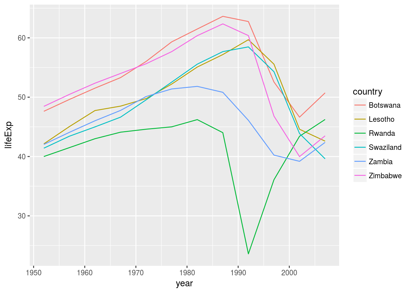
25.2.4 25.2.5 Exercises
- A linear trend seems to be slightly too simple for the overall trend. Can you do better with a quadratic polynomial? How can you interpret the coefficients of the quadratic? (Hint you might want to transform
yearso that it has mean zero.)
modquad <- function(df){
  lm(data = df, lifeExp ~ poly(year,2))
}

quad <- gapminder %>%
  mutate(year = year - mean(year)) %>%
  group_by(country)%>%
  nest()%>%
  mutate(model = purrr::map(data,modquad))

quad <- quad %>%
  mutate(resids = map2(data, model, add_residuals)
         # data here is the column name, so is model.
         )
unnest(quad,resids)
## # A tibble: 1,704 x 7
## country continent year lifeExp pop gdpPercap resid
## <fctr> <fctr> <dbl> <dbl> <int> <dbl> <dbl>
## 1 Afghanistan Asia -27.5 28.801 8425333 779.4453 0.6223132
## 2 Afghanistan Asia -22.5 30.332 9240934 820.8530 -0.1662073
## 3 Afghanistan Asia -17.5 31.997 10267083 853.1007 -0.6321523
## 4 Afghanistan Asia -12.5 34.020 11537966 836.1971 -0.5515220
## 5 Afghanistan Asia -7.5 36.088 13079460 739.9811 -0.2373162
## 6 Afghanistan Asia -2.5 38.438 14880372 786.1134 0.5474650
## 7 Afghanistan Asia 2.5 39.854 12881816 978.0114 0.5868217
## 8 Afghanistan Asia 7.5 40.822 13867957 852.3959 0.3667537
## 9 Afghanistan Asia 12.5 41.674 16317921 649.3414 0.2192612
## 10 Afghanistan Asia 17.5 41.763 22227415 635.3414 -0.5026558
## # ... with 1,694 more rowsCheck the residuals
unnest(quad, resids) %>%
ggplot(aes(group = country))+
geom_line(aes(x = year, y = resid))+
facet_wrap(~continent, nrow = 2)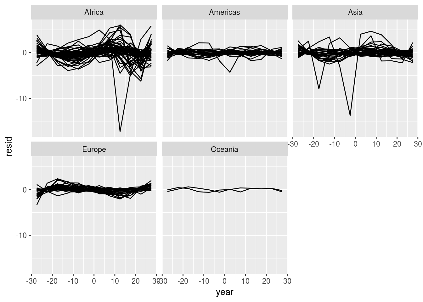 Check the quality
quad %>%
  mutate(glance = map(model, broom::glance))%>%
  unnest(glance, .drop = TRUE)%>%
  arrange(r.squared)
## # A tibble: 142 x 12
## country r.squared adj.r.squared sigma statistic
## <fctr> <dbl> <dbl> <dbl> <dbl>
## 1 Rwanda 0.01735115 -0.2010153 6.912349 0.07945888
## 2 Liberia 0.61279138 0.5267450 1.664180 7.12164206
## 3 Uganda 0.64045980 0.5605620 2.484068 8.01598555
## 4 Cambodia 0.68205481 0.6114003 5.567185 9.65338275
## 5 Botswana 0.69396257 0.6259542 3.626425 10.20408358
## 6 Lesotho 0.70356998 0.6376966 3.559901 10.68064850
## 7 Zimbabwe 0.71095742 0.6467257 4.203267 11.06864030
## 8 Zambia 0.72850734 0.6681756 2.565257 12.07503373
## 9 Congo, Dem. Rep. 0.72952938 0.6694248 1.649671 12.13766664
## 10 Swaziland 0.73107550 0.6713145 3.762450 12.23332097
## # ... with 132 more rows, and 7 more variables: p.value <dbl>, df <int>,
## # logLik <dbl>, AIC <dbl>, BIC <dbl>, deviance <dbl>, df.residual <int>Compare to the linear model, the r.squared is much better.
quad %>%
  mutate(glance = map(model, broom::glance))%>%
  unnest(glance, .drop = TRUE) %>%
  ggplot(aes(r.squared)) +
  geom_histogram(bins = 100)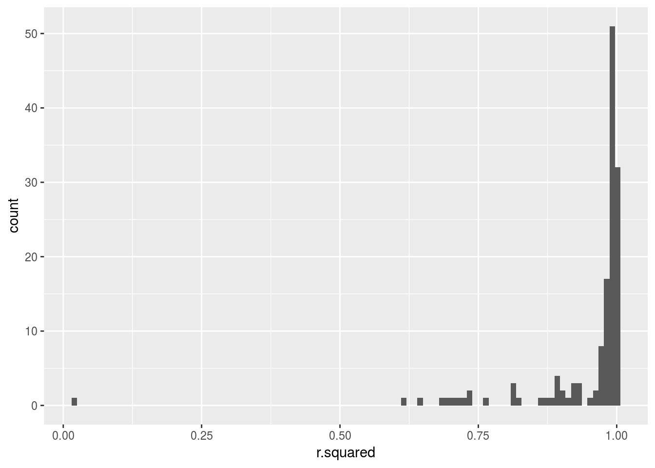
- Explore other methods for visualising the distribution of
R^2per continent. You might want to try theggbeeswarmpackage, which provides similar methods for avoiding overlaps as jitter, but uses deterministic methods.
library(ggbeeswarm)
gapminder %>%
mutate(year = year - mean(year)) %>%
group_by(continent,country)%>%
nest() %>%
mutate(model = map(data, modquad)) %>%
mutate(glance = map(model, broom::glance))%>%
unnest(glance) %>%
ggplot(aes(x= continent, y =r.squared,color = continent)) +
geom_beeswarm()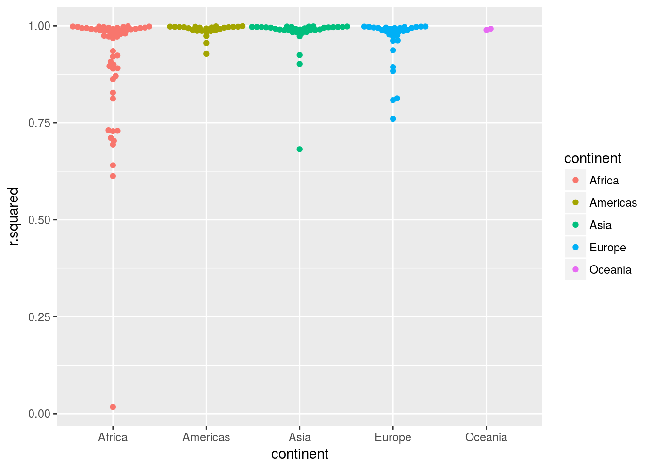 It is clear that many Africa countries have patterns not captured by the polynomial functions.
3.To create the last plot (showing the data for the countries with the worst model fits), we needed two steps: we created a data frame with one row per country and then semi-joined it to the original dataset. It’s possible avoid this join if we use nnest() instead of unnest(.drop = TRUE). How?
gapminder %>%
  mutate(year = year - mean(year)) %>%
  group_by(country)%>%
  nest() %>%
  mutate(model = map(data, modquad)) %>%
  mutate(glance = map(model, broom::glance))%>%
  unnest(glance) %>%
  unnest(data) %>%
  semi_join(gapminder, by = c("pop","country")) %>%
  arrange(r.squared) %>%
  filter(r.squared %in% unique(r.squared)[1:6])%>%
  ggplot(aes(x = year + mean(gapminder$year), y = log(pop) )) +
  geom_line(aes(color = country))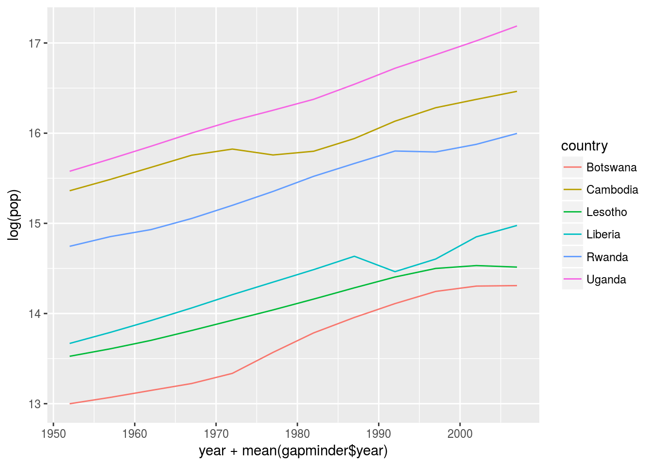
25.3 List-columns
Note: The meaning of list-columns is a column as a list contains arbitary data structure you want.
# example of creating a list-columns
tibble(
  x = list(1:3,3:5),
  y = list(letters[1:4],as.factor(letters[5:9]))
)
## # A tibble: 2 x 2
## x y
## <list> <list>
## 1 <int [3]> <chr [4]>
## 2 <int [3]> <fctr [5]>25.4 Creating list-columns
Note: 1. tidyr::nest() to convert a grouped data frame into nested data frame. 2. mutate() with vectorised functions. 3. summarise() with summary functions
25.4.0.1 With nesting
25.4.0.2 From vectorised functions
df <- tribble(
  ~x1,
  "a,b,c",
  "d,e,f,g"
)
df %>%
  mutate(x2 = stringr::str_split(x1, ","))
## # A tibble: 2 x 2
## x1 x2
## <chr> <list>
## 1 a,b,c <chr [3]>
## 2 d,e,f,g <chr [4]>purrr::invoke_map is a powerful function that you get a function and pass a list of parameters to it.
sim <- tribble(
  ~f,      ~params,
  "runif", list(min = -1, max = -1),
  "rnorm", list(sd = 5),
  "rpois", list(lambda = 10)
)

sim %>%
  mutate(sims = invoke_map(f, params, n = 10))
## # A tibble: 3 x 3
## f params sims
## <chr> <list> <list>
## 1 runif <list [2]> <dbl [10]>
## 2 rnorm <list [1]> <dbl [10]>
## 3 rpois <list [1]> <int [10]>rm(list = ls())
sim <- tibble::tribble(
~f, ~params,
"runif", list(min = -1, max = -1),
"rnorm", list(sd = 5),
"rpois", list(lambda = 10)
)%>%
mutate(sims = purrr::invoke_map(f, params, n = 10))mydata <-
tibble(col_a = rep(c("a", "b"), 5)) %>%
mutate(col_b = map(col_a, function (x) { list(a = x, b = x, c = x) }))
mydata%>%
filter (col_a == "a")## # A tibble: 5 x 2
## col_a col_b
## <chr> <list>
## 1 a <list [3]>
## 2 a <list [3]>
## 3 a <list [3]>
## 4 a <list [3]>
## 5 a <list [3]>mydata <-
tibble(col_a = rep(c("a", "b"), 5)) %>%
mutate(col_b = map(col_a, function (x) { list(a = x, b = x, c = x) }))%>%
filter (col_a == "a")
class(mydata)## [1] "tbl_df" "tbl" "data.frame"25.4.0.3 From multivalued summaries
See quantile()
25.4.0.4 From a named list
See enframe()
25.4.5 Exercises
- List all the functions that you can think of that take a atomic vector and return a list.
quantile is an example
- Brainstorm useful summary functions that, like
quantile(), return multiple values.
You can write one for example as the example I constructed from answers based on this post
df <- data.frame(group=c('A','A','A','A','B','B','B','B','C','C','C','C'), x=rnorm(12,1,1), y=rnorm(12,1,1))
f <- function(x,y) list(setNames(coef(lm(x ~ y)), c("a", "b")))
df %>%
  group_by(group)%>%
  summarise(coef = f(x,y))
## # A tibble: 3 x 2
## group coef
## <fctr> <list>
## 1 A <dbl [2]>
## 2 B <dbl [2]>
## 3 C <dbl [2]>- What’s missing in the following data frame? How does
quantile()return that missing piece? Why isn’t that helpful here?
Not sure what the question is asking for.
- What does this code do? Why might might it be useful?
I slightly modified the code to make its behavior more explicit
myfun <- function(x){
  list(quantile(x))
}

mtcars %>%
  group_by(cyl) %>%
  summarise_each(funs(myfun))
This code apply the list function to each variable of the grouped data frames. This may be useful if you want to apply different summarize functions to different columns. Here we just use the same function list.
25.5 Simplifying list-columns
25.5.1 List to vector
df <- tribble(
  ~x,
  letters[1:5],
  1:3,
  runif(5)
)
purrr::map_char takes a column whose element is a list and map each list to a char using provided function. Similar ideas apply for map_int, etc.
25.5.2 Unnest
unnesting two columns simultaneously requires they have exactly the same shape. The following code fails
df2 <- tribble(
  ~x, ~y,           ~z,
   1, "a",         1:2,
   2, c("b", "c"),   3
)
df2 %>% unnest(y, z)
25.5.3 Exercises
- Why might the
lengths()function be useful for creating atomic vector columns from list-columns?
Because you can’t use count directly and lengths() is equivalent to the n() when the data frame is not nested.
The following three ways all calculate the number of observables in each group.
df <- data.frame(group=c('A','A','A','A','B','B','B','B','C','C','C','C'), x=rnorm(12,1,1), y=rnorm(12,1,1))

df %>%
  group_by(group)%>%
  summarize(n = n())
## # A tibble: 3 x 2
## group n
## <fctr> <int>
## 1 A 4
## 2 B 4
## 3 C 4df %>%
group_by(group)%>%
nest() %>%
mutate(
n = map_int(data,nrow)
)## # A tibble: 3 x 3
## group data n
## <fctr> <list> <int>
## 1 A <tibble [4 x 2]> 4
## 2 B <tibble [4 x 2]> 4
## 3 C <tibble [4 x 2]> 4df %>%
group_by(group) %>%
summarize_each(funs(list)) %>%
mutate(n = map_int(x,length))## `summarise_each()` is deprecated.
## Use `summarise_all()`, `summarise_at()` or `summarise_if()` instead.
## To map `funs` over all variables, use `summarise_all()`## # A tibble: 3 x 4
## group x y n
## <fctr> <list> <list> <int>
## 1 A <dbl [4]> <dbl [4]> 4
## 2 B <dbl [4]> <dbl [4]> 4
## 3 C <dbl [4]> <dbl [4]> 4- List the most common types of vector found in a data frame. What makes lists different?
- bool
- numeric
- integer
- factor
- char List is special because it is nested, a list can contain other lists and any other kind of elements.
25.6 Making tidy data with broom
Note:
To turn models into tidy data frames
broom::glance(model)broom::tidy(mdoel)broom::augment(model,data)