Chapter 5 Rating Scale Model
5.1 Rasch Rating Scale Model
The Rasch Rating Scale Model (RSM; sometimes also called the Polytomous Rasch model) was developed by Andrich(1978) for polytomous data (data with >= 2 ordinal categories). It provides estimates of a; Person locations, b; Item Difficulties and c; An overall set of thresholds (fixed across items).
Rating Scale Model Equation
\[ln\left[\frac{P_{n_i(x=k)}}{P_{n_i(x=k-1)}}\right]=\theta_{n}-\delta_{i}-\tau_{k}\] Where \(\theta\) is the person’s ability, \(\delta\) is the item’s difficulty, and \(\tau\) is the thresholds which are estimated empirically for the whole set of items. The RSM assumes that the threshold structure is fixed across items. The relative distance between thresholds is the same across items, but items still have different difficulties. The thresholds just move up or down the logit scale.
5.2 R-Lab: Rasch Rating Scale Model with “eRm” package
5.2.1 Load the packages that required for the Rasch Rating Scale Analysis
5.2.2 Information about the data
We are going to practice running the Rating Scale (RS) model using the “TAM” package. Specifically, we will be working with data from a writing assessment in which students received polytomous ratings on essays. Several researchers have used this dataset in published studies, and it is considered a classic example of rating data.
The original data collection design is described by Braun(1988). The original dataset includes ratings for 32 students by 12 raters on three separate essay compositions. For this lab, we will look at the data from Essay 1. For ease of interpretation, the essay ratings from the original dataset have been recoded from nine categories to three categories (1 = low achievement, 2 = middle achievement; 3 = high achievement).
In our analysis, we will treat the 12 raters as 12 polytomous “items” that share the three-category rating scale structure. Raters with high “difficulty” calibrations can be interpreted as severe – these raters assign low scores more often. Raters with low “difficulty” calibrations can be interpreted as lenient – these raters assign high scores more often.
5.2.3 Get Data Prepared
we will try running a polytomous Rasch model using some of the example data that is provided with the TAM package.
*Note If you want to use the “eRm” package to run the Rating Scale model, you need to make sure that each item has responses in the same categories as each of the other items.
##   Student rater_1 rater_2 rater_3 rater_4 rater_5 rater_6 rater_7 rater_8
## 1       1       2       2       1       2       3       2       3       3
## 2       2       2       2       2       2       2       1       2       2
## 3       3       2       1       2       2       2       2       1       2
## 4       4       1       2       2       2       1       2       1       1
## 5       5       2       2       1       2       2       3       2       2
## 6       6       2       2       2       3       2       2       3       2
##   rater_9 rater_10 rater_11 rater_12
## 1       3        2        3        3
## 2       2        2        1        2
## 3       1        2        2        2
## 4       1        2        2        2
## 5       2        2        2        2
## 6 1 2 2 2## Student rater_1 rater_2 rater_3 rater_4
## Min. : 1.00 Min. :1.000 Min. :1.00 Min. :1.000 Min. :1.00
## 1st Qu.: 8.75 1st Qu.:1.750 1st Qu.:1.75 1st Qu.:1.000 1st Qu.:2.00
## Median :16.50 Median :2.000 Median :2.00 Median :2.000 Median :2.00
## Mean :16.50 Mean :1.781 Mean :1.75 Mean :1.688 Mean :2.25
## 3rd Qu.:24.25 3rd Qu.:2.000 3rd Qu.:2.00 3rd Qu.:2.000 3rd Qu.:3.00
## Max. :32.00 Max. :3.000 Max. :2.00 Max. :3.000 Max. :3.00
## rater_5 rater_6 rater_7 rater_8
## Min. :1.000 Min. :1.000 Min. :1.000 Min. :1.000
## 1st Qu.:2.000 1st Qu.:1.750 1st Qu.:1.000 1st Qu.:1.000
## Median :2.000 Median :2.000 Median :2.000 Median :2.000
## Mean :1.875 Mean :1.812 Mean :1.969 Mean :1.688
## 3rd Qu.:2.000 3rd Qu.:2.000 3rd Qu.:3.000 3rd Qu.:2.000
## Max. :3.000 Max. :3.000 Max. :3.000 Max. :3.000
## rater_9 rater_10 rater_11 rater_12
## Min. :1.000 Min. :1.000 Min. :1.000 Min. :1.000
## 1st Qu.:1.000 1st Qu.:2.000 1st Qu.:2.000 1st Qu.:2.000
## Median :2.000 Median :2.000 Median :2.000 Median :2.000
## Mean :1.875 Mean :2.031 Mean :1.938 Mean :2.094
## 3rd Qu.:2.000 3rd Qu.:2.000 3rd Qu.:2.000 3rd Qu.:2.000
## Max. :3.000 Max. :3.000 Max. :3.000 Max. :3.0005.2.4 Run the Rating Scale Model
## ------------------------------------------------------------
## TAM 3.5-19 (2020-05-05 22:45:39)
## R version 3.6.2 (2019-12-12) x86_64, linux-gnu | nodename=bookdown | login=unknown
##
## Date of Analysis: 2021-01-05 19:53:47
## Time difference of 3.102939 secs
## Computation time: 3.102939
##
## Multidimensional Item Response Model in TAM
##
## IRT Model: RSM
## Call:
## TAM::tam.mml(resp = rs_data, irtmodel = "RSM")
##
## ------------------------------------------------------------
## Number of iterations = 1000
## Numeric integration with 21 integration points
##
## Deviance = 554.34
## Log likelihood = -277.17
## Number of persons = 32
## Number of persons used = 32
## Number of items = 12
## Number of estimated parameters = 15
##     Item threshold parameters = 14
##     Item slope parameters = 0
##     Regression parameters = 0
##     Variance/covariance parameters = 1
##
## AIC = 584  | penalty=30    | AIC=-2*LL + 2*p
## AIC3 = 599  | penalty=45    | AIC3=-2*LL + 3*p
## BIC = 606  | penalty=51.99    | BIC=-2*LL + log(n)*p
## aBIC = 558  | penalty=3.35    | aBIC=-2*LL + log((n-2)/24)*p  (adjusted BIC)
## CAIC = 621  | penalty=66.99    | CAIC=-2*LL + [log(n)+1]*p  (consistent AIC)
## AICc = 614  | penalty=60    | AICc=-2*LL + 2*p + 2*p*(p+1)/(n-p-1)  (bias corrected AIC)
## GHP = 0.76085     | GHP=( -LL + p ) / (#Persons * #Items)  (Gilula-Haberman log penalty)
##
## ------------------------------------------------------------
## EAP Reliability
## [1] 0.805
## ------------------------------------------------------------
## Covariances and Variances
##       [,1]
## [1,] 1.579
## ------------------------------------------------------------
## Correlations and Standard Deviations (in the diagonal)
##       [,1]
## [1,] 1.257
## ------------------------------------------------------------
## Regression Coefficients
##      [,1]
## [1,]    0
## ------------------------------------------------------------
## Item Parameters -A*Xsi
##        item  N     M xsi.item AXsi_.Cat1 AXsi_.Cat2 AXsi_.Cat3 B.Cat1.Dim1
## 1   rater_1 32 1.781   -2.563     -9.627    -10.777     -7.688           1
## 2   rater_2 32 1.750   -5.672     -9.911    -11.343         NA           1
## 3   rater_3 32 1.688   -2.146     -9.211     -9.944     -6.439           1
## 4   rater_4 32 2.250   -4.638    -11.702    -14.927    -13.913           1
## 5   rater_5 32 1.875   -2.978    -10.043    -11.608     -8.934           1
## 6   rater_6 32 1.812   -2.701     -9.766    -11.054     -8.104           1
## 7   rater_7 32 1.969   -3.394    -10.458    -12.439    -10.181           1
## 8   rater_8 32 1.688   -2.146     -9.211     -9.944     -6.439           1
## 9   rater_9 32 1.875   -2.978    -10.043    -11.608     -8.934           1
## 10 rater_10 32 2.031   -3.671    -10.735    -12.993    -11.012           1
## 11 rater_11 32 1.938   -3.255    -10.320    -12.162     -9.765           1
## 12 rater_12 32 2.094   -3.947    -11.012    -13.546    -11.842           1
##    B.Cat2.Dim1 B.Cat3.Dim1
## 1            2           3
## 2            2           0
## 3            2           3
## 4            2           3
## 5            2           3
## 6            2           3
## 7            2           3
## 8            2           3
## 9            2           3
## 10           2           3
## 11           2           3
## 12           2           3
##
## Item Parameters Xsi
##             xsi se.xsi
## rater_1  -2.563  0.372
## rater_2  -2.846  0.460
## rater_3  -2.146  0.373
## rater_4  -4.638  0.372
## rater_5  -2.978  0.372
## rater_6  -2.701  0.372
## rater_7  -3.394  0.372
## rater_8  -2.146  0.373
## rater_9  -2.978  0.372
## rater_10 -3.671  0.372
## rater_11 -3.256  0.372
## rater_12 -3.948  0.372
## Cat1     -7.065  0.182
## Cat2      1.414  0.116
##
## Item Parameters in IRT parameterization
##        item alpha   beta tau.Cat1 tau.Cat2 tau.Cat3
## 1   rater_1     1 -2.563   -7.065    1.413    5.652
## 2   rater_2     1 -5.672   -4.239    4.239       NA
## 3   rater_3     1 -2.146   -7.065    1.413    5.652
## 4   rater_4     1 -4.638   -7.065    1.413    5.652
## 5   rater_5     1 -2.978   -7.065    1.413    5.652
## 6   rater_6     1 -2.701   -7.065    1.413    5.652
## 7   rater_7     1 -3.394   -7.065    1.413    5.652
## 8   rater_8     1 -2.146   -7.065    1.413    5.652
## 9   rater_9     1 -2.978   -7.065    1.413    5.652
## 10 rater_10     1 -3.671   -7.065    1.413    5.652
## 11 rater_11     1 -3.255   -7.065    1.413    5.652
## 12 rater_12     1 -3.947   -7.065    1.413    5.652
5.2.5 Wright Map & Expected Response Curves & Item characteristic curves
Wright Map or Variable Map
# Plot the Variable Map
graphics.off() # In case you can not run the plot correctly
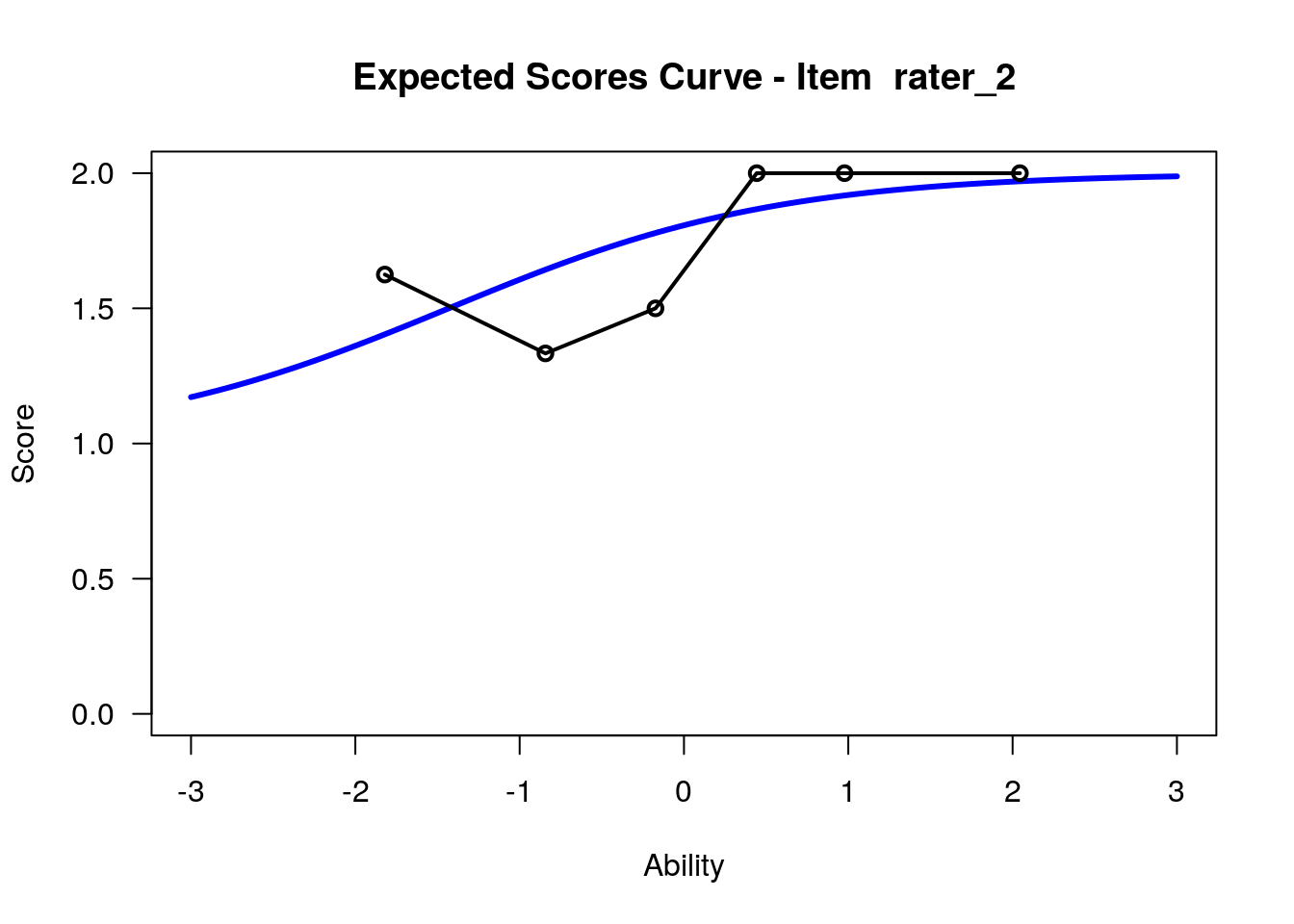
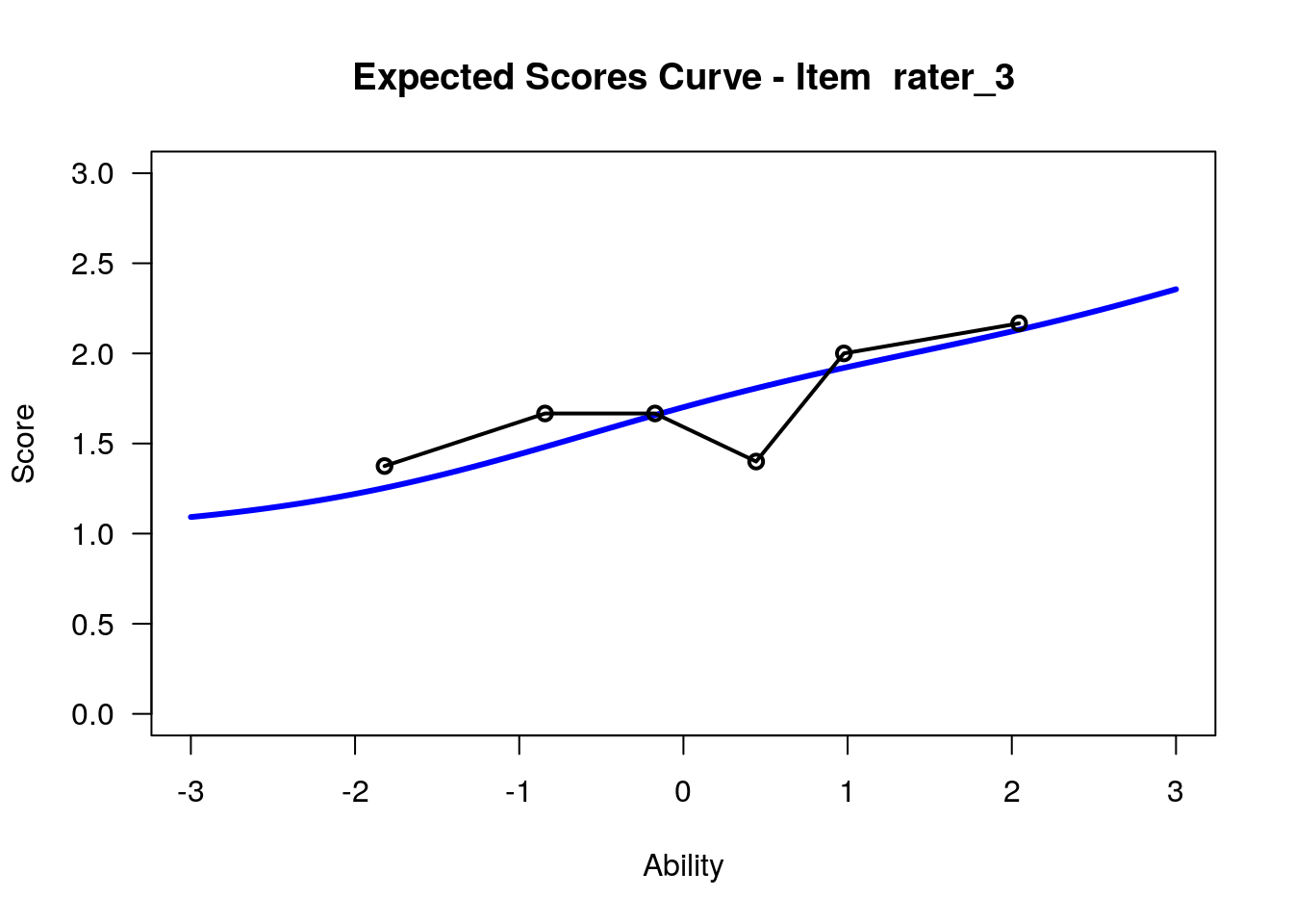
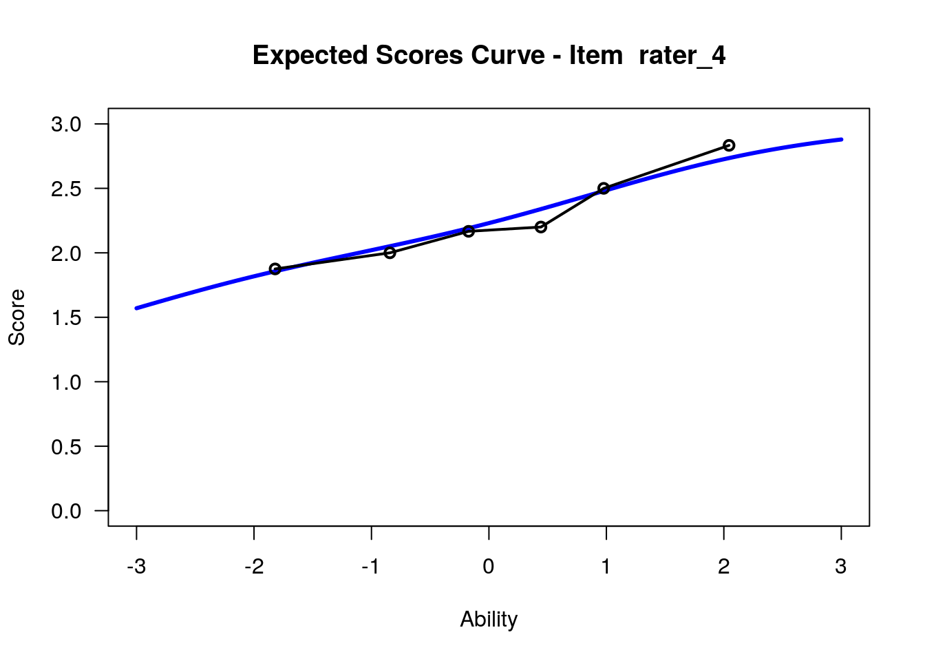
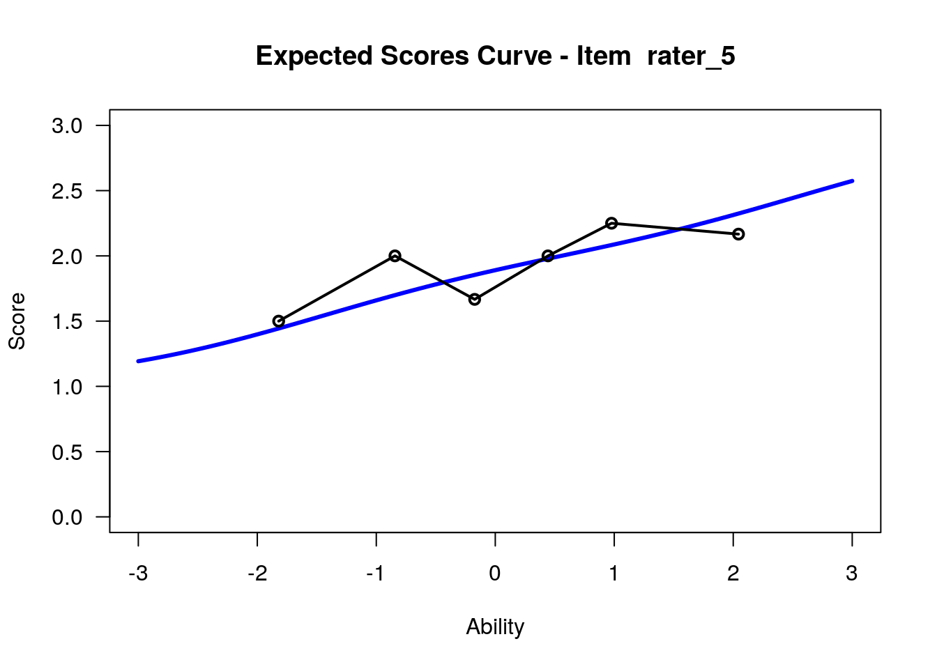
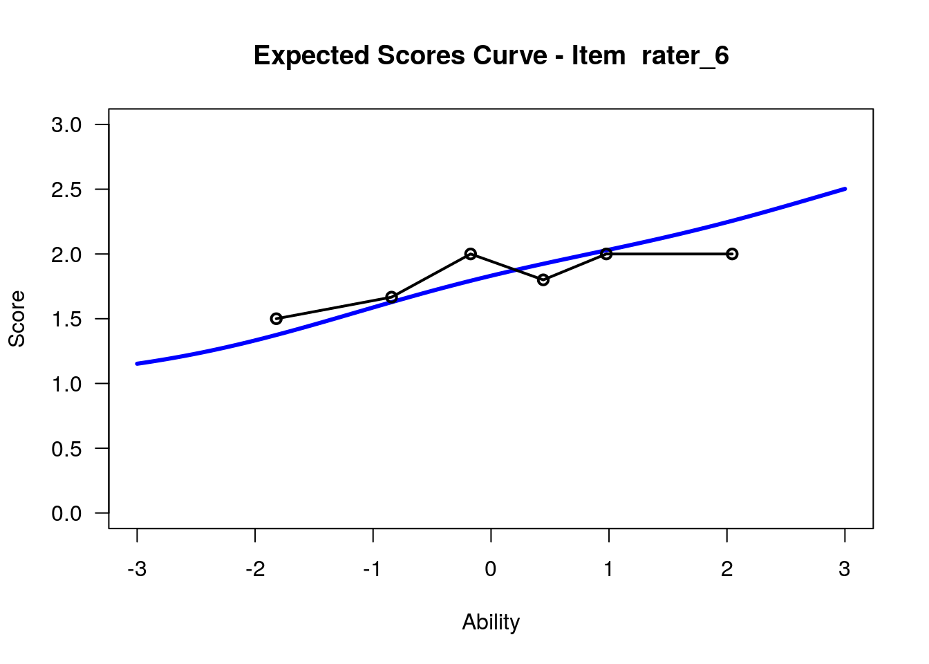
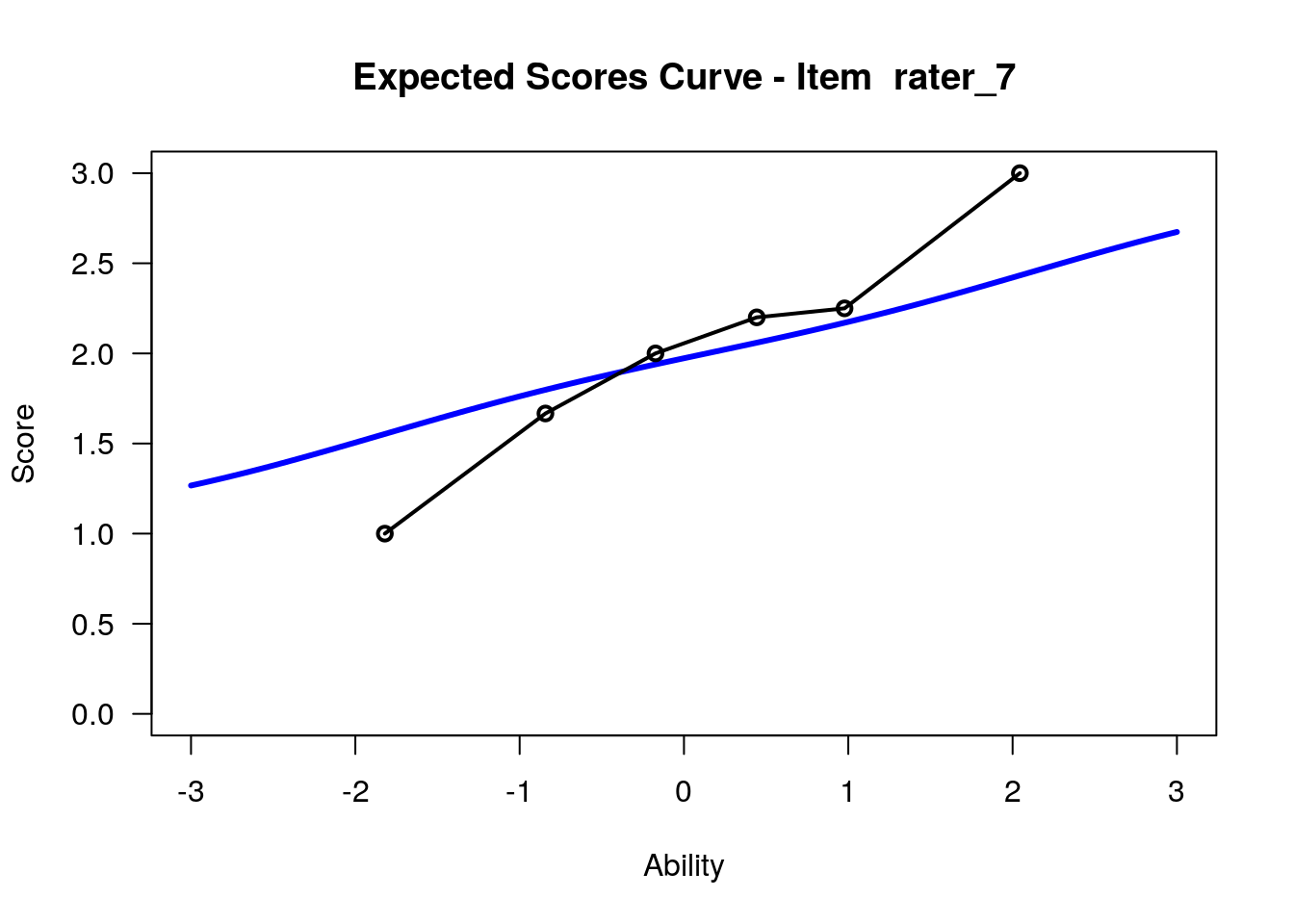
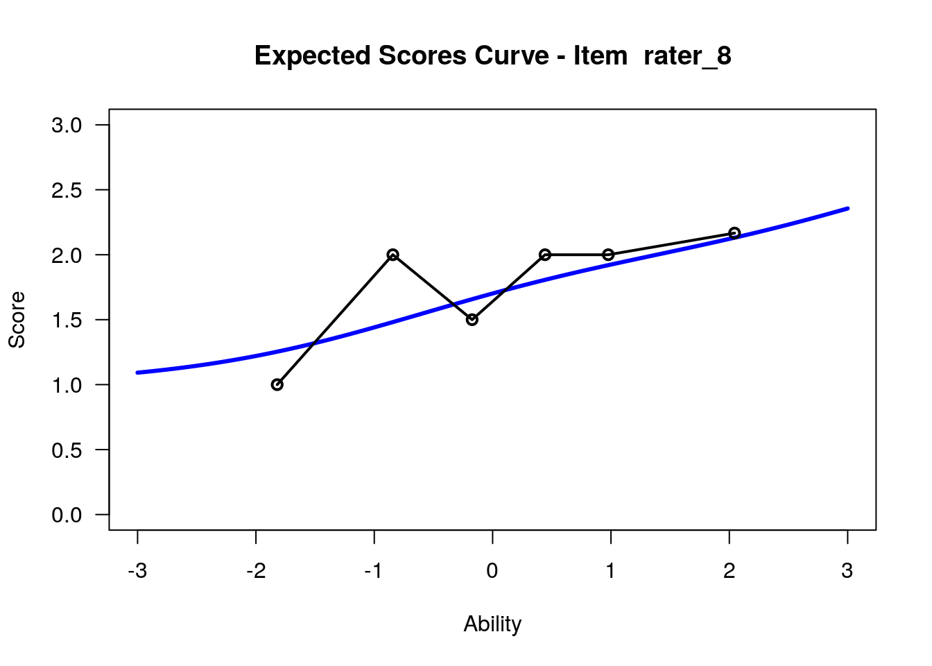
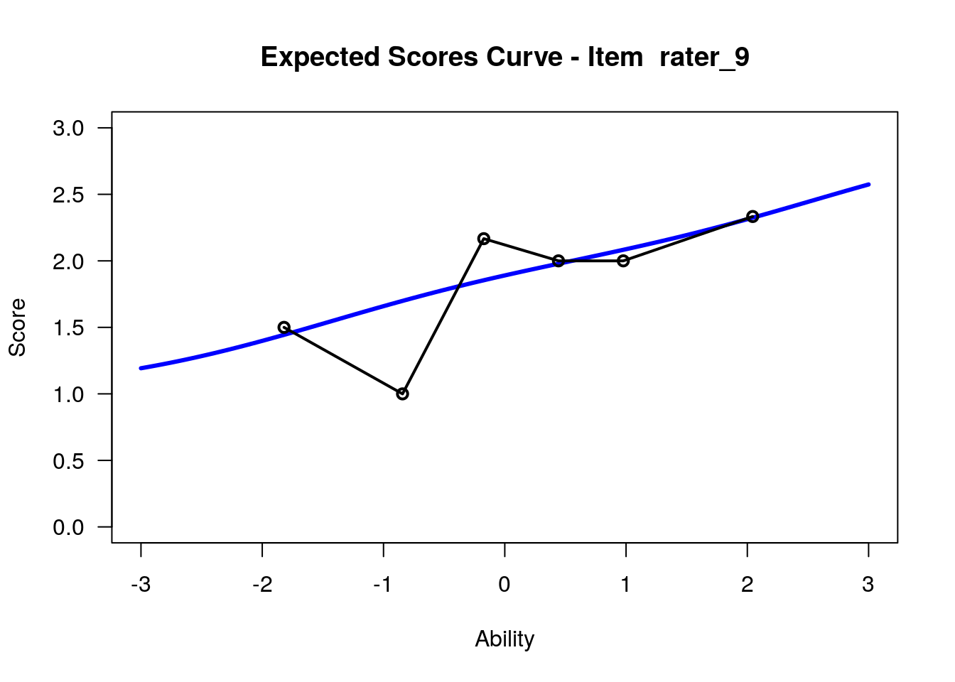
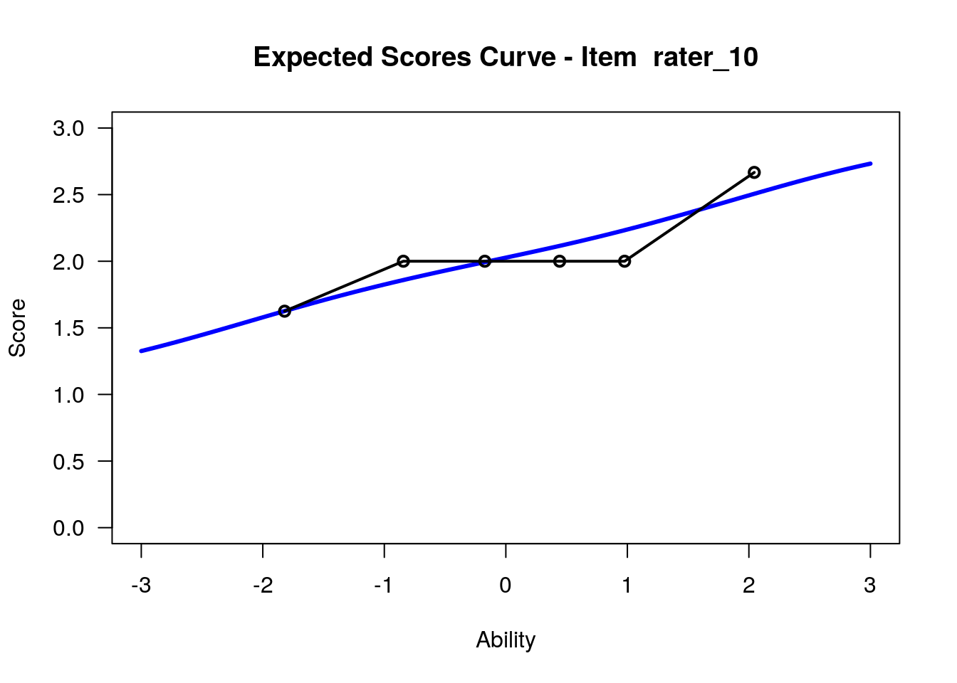
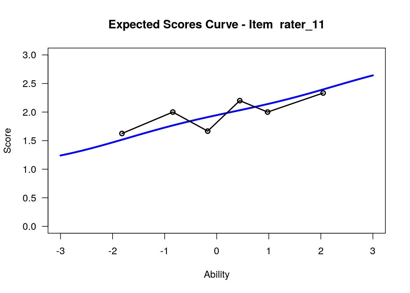
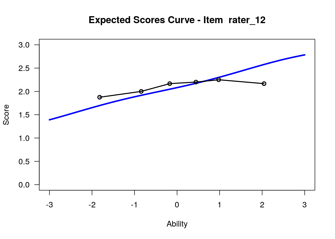
IRT.WrightMap(rs_model,show.thr.lab=TRUE) Expected Response Curves
## Iteration in WLE/MLE estimation  1   | Maximal change  2.716
## Iteration in WLE/MLE estimation  2   | Maximal change  0.2947
## Iteration in WLE/MLE estimation  3   | Maximal change  0.0264
## Iteration in WLE/MLE estimation  4   | Maximal change  0.0014
## Iteration in WLE/MLE estimation  5   | Maximal change  1e-04
## ----
##  WLE Reliability= 0.808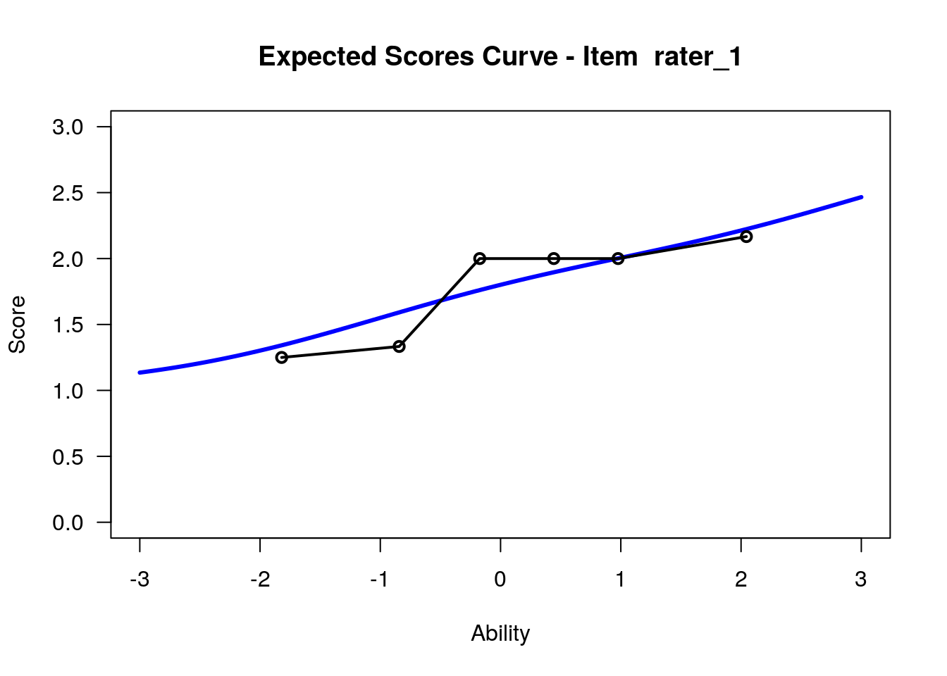
## ....................................................
##  Plots exported in png format into folder:
##  /opt/rstudio-connect/mnt/report/Plots
Item characteristic curves (but now as thresholds)
## Iteration in WLE/MLE estimation  1   | Maximal change  2.716
## Iteration in WLE/MLE estimation  2   | Maximal change  0.2947
## Iteration in WLE/MLE estimation  3   | Maximal change  0.0264
## Iteration in WLE/MLE estimation  4   | Maximal change  0.0014
## Iteration in WLE/MLE estimation  5   | Maximal change  1e-04
## ----
##  WLE Reliability= 0.808
## ....................................................
## Plots exported in png format into folder:
## /opt/rstudio-connect/mnt/report/Plots5.2.6 Item estimates and fit Statistics
# We can use the similar code to achieve the item estimate as what we did for the Dichotomous Analysis
graphics.off()
rs_model$xsi # The first column is the item difficulty. In this case, is the rater's rating severity.
## xsi se.xsi
## rater_1 -2.562786 0.3721864
## rater_2 -2.845848 0.4595648
## rater_3 -2.146289 0.3732464
## rater_4 -4.638103 0.3716336
## rater_5 -2.978494 0.3721616
## rater_6 -2.701294 0.3721176
## rater_7 -3.394130 0.3722341
## rater_8 -2.146289 0.3732464
## rater_9 -2.978494 0.3721616
## rater_10 -3.671164 0.3720920
## rater_11 -3.255568 0.3722386
## rater_12 -3.947827 0.3718025
## Cat1 -7.064972 0.1818587
## Cat2 1.413518 0.1156938## Item fit calculation based on 100 simulations
## |**********|
## |----------|## $itemfit
## parameter Outfit Outfit_t Outfit_p Outfit_pholm Infit
## 1 rater_1 0.5412197 -2.22437362 0.026123318 0.31347981 0.5728601
## 2 rater_2 0.9921955 -0.01305309 0.989585435 1.00000000 1.1396166
## 3 rater_3 1.3339648 1.36221289 0.173130708 1.00000000 1.3010337
## 4 rater_4 0.7567609 -1.07179625 0.283811557 1.00000000 0.7602385
## 5 rater_5 0.7728834 -0.91355944 0.360948386 1.00000000 0.7803290
## 6 rater_6 1.1240013 0.55247755 0.580621209 1.00000000 1.1167225
## 7 rater_7 1.5331164 1.86014503 0.062865010 0.69151511 1.5205183
## 8 rater_8 0.9599078 -0.11360257 0.909552851 1.00000000 0.9676102
## 9 rater_9 1.8483264 2.77674351 0.005490649 0.07686908 1.8085516
## 10 rater_10 0.5858305 -1.85328666 0.063841282 0.69151511 0.6235676
## 11 rater_11 0.8026202 -0.75986923 0.447332757 1.00000000 0.7999848
## 12 rater_12 0.6564147 -1.49298769 0.135440410 1.00000000 0.6641154
## 13 Cat1 0.9936559 -0.31811202 0.750399963 1.00000000 1.1523215
## 14 Cat2 1.1262090 2.26157958 0.023723391 0.30840408 1.1113940
## Infit_t Infit_p Infit_pholm
## 1 -2.02717750 0.042644263 0.5543754
## 2 0.61940708 0.535648220 1.0000000
## 3 1.24788175 0.212074365 1.0000000
## 4 -1.04787758 0.294695015 1.0000000
## 5 -0.87466882 0.381754131 1.0000000
## 6 0.52705210 0.598157412 1.0000000
## 7 1.82352661 0.068223670 0.7504604
## 8 -0.07556766 0.939763064 1.0000000
## 9 2.67193552 0.007541514 0.1055812
## 10 -1.64272848 0.100439123 1.0000000
## 11 -0.76953728 0.441574420 1.0000000
## 12 -1.44652336 0.148030466 1.0000000
## 13 1.02465277 0.305527057 1.0000000
## 14 1.98694473 0.046928522 0.5631423
##
## $time
## [1] "2021-01-05 19:53:52 UTC" "2021-01-05 19:53:52 UTC"
##
## $CALL
## tam.fit(tamobj = rs_model)
##
## attr(,"class")
## [1] "tam.fit"# Note the last two rows also provides you the average fit statistics for category 1 and category 2. For this analysis, we are not focus on these data.
# We can also check the Rating Scale Thresholds
rs_threshold <- tam.threshold(rs_model)
rs_threshold # This provides the detail logit location for each categories for each rater.## Cat1 Cat2 Cat3
## rater_1 -9.627960 -1.1631775 3.102814
## rater_2 -9.911041 -1.4321594 NA
## rater_3 -9.211395 -0.7466125 3.519379
## rater_4 -11.703278 -3.2384949 1.027496
## rater_5 -10.043610 -1.5788269 2.687164
## rater_6 -9.766388 -1.3017883 2.964203
## rater_7 -10.459259 -1.9944763 2.271515
## rater_8 -9.211395 -0.7466125 3.519379
## rater_9 -10.043610 -1.5788269 2.687164
## rater_10 -10.736298 -2.2715149 1.994476
## rater_11 -10.320831 -1.8560486 2.409943
## rater_12 -11.012970 -2.5481873 1.717804Note The tam.threshold() function is actually calculating Thurstonian thresholds, whereas the tau estimates are Andrich thresholds. These are different parameters.
The Thurstonian thresholds are cumulative, meaning that they reflect the probability for responding in a category of interest or any higher category. The Andrich thresholds are adjacent-categories thresholds, which reflect the point on the logit scale at which there is an equal probability for a rating in a category of interest or the category just below it. You can check here for more information.
5.2.7 Person estimates and fit Statistics
## Iteration in WLE/MLE estimation  1   | Maximal change  2.716
## Iteration in WLE/MLE estimation  2   | Maximal change  0.2947
## Iteration in WLE/MLE estimation  3   | Maximal change  0.0264
## Iteration in WLE/MLE estimation  4   | Maximal change  0.0014
## Iteration in WLE/MLE estimation  5   | Maximal change  1e-04
## ----
## WLE Reliability= 0.808## [1] 2.4085783 -0.3688909 -0.7300439 -1.3964450 0.4427846 0.8732767rs_personfit <- tam.personfit(rs_model)
# Check the first 6 students' person fit statistics
head(rs_personfit)## outfitPerson outfitPerson_t infitPerson infitPerson_t
## 1 1.6895293 1.12430028 1.7074016 2.06808271
## 2 0.6906362 -0.64320564 0.7046442 -0.63946517
## 3 0.8893534 -0.16892776 0.9011214 -0.16041221
## 4 0.8501677 -0.43608082 0.8718146 -0.39029650
## 5 0.8118033 -0.20983489 0.8377828 -0.16789359
## 6 0.9185230 0.02208877 0.9538410 0.071275655.3 Another Example with “eRm” package
The “eRm” package also provide the function to run a polytomous Rasch model. In this example, we will use a build-in data set in “eRm” package as an example.
5.3.1 Load the example data
### Load the example data:
data("rsmdat")
# These data include 20 participants’ responses to six items that included four ordered categories (0, 1, 2, and 3).
summary(rsmdat)
## I1 I2 I3 I4 I5
## Min. :0.00 Min. :0 Min. :0.00 Min. :0.00 Min. :0.0
## 1st Qu.:0.75 1st Qu.:0 1st Qu.:0.00 1st Qu.:0.00 1st Qu.:0.0
## Median :1.50 Median :1 Median :1.00 Median :1.00 Median :2.0
## Mean :1.35 Mean :1 Mean :1.05 Mean :1.25 Mean :1.5
## 3rd Qu.:2.00 3rd Qu.:2 3rd Qu.:2.00 3rd Qu.:2.00 3rd Qu.:3.0
## Max. :3.00 Max. :3 Max. :3.00 Max. :3.00 Max. :3.0
## I6
## Min. :0.00
## 1st Qu.:0.75
## Median :2.00
## Mean :1.80
## 3rd Qu.:3.00
## Max. :3.00Important! Note that in the summary of the “rsmdat” object, there are responses in all 4 categories for all items. This means that it is possible to run the Rating Scale model on these item responses. If participants did not use all of the categories on all of the items, then we would need to run the Partial Credit model instead.
5.3.3 Examine item difficulty and threshold SEs
##
## Design Matrix Block 1:
##    Location Threshold 1 Threshold 2 Threshold 3
## I1  0.02202    -0.02395    -0.19134     0.28135
## I2  0.35112     0.30515     0.13776     0.61045
## I3  0.30183     0.25586     0.08847     0.56116
## I4  0.11328     0.06731    -0.10009     0.37261
## I5 -0.11417    -0.16013    -0.32753     0.14517
## I6 -0.39828    -0.44424    -0.61164    -0.13894
## thresh beta I1.c1 thresh beta I1.c2 thresh beta I1.c3 thresh beta I2.c1
## 0.1954895 0.4973730 0.4474697 0.2053695
## thresh beta I2.c2 thresh beta I2.c3 thresh beta I3.c1 thresh beta I3.c2
## 0.5154307 0.4784415 0.2028161 0.5120890
## thresh beta I3.c3 thresh beta I4.c1 thresh beta I4.c2 thresh beta I4.c3
## 0.4735296 0.1965073 0.5013598 0.4556107
## thresh beta I5.c1 thresh beta I5.c2 thresh beta I5.c3 thresh beta I6.c1
## 0.1965178 0.4929850 0.4359921 0.2084872
## thresh beta I6.c2 thresh beta I6.c3
## 0.4901538 0.41540925.3.4 Examine Person locations (theta) and SEs
# Standard errors for theta estimates:
person.locations.estimate <- person.parameter(rs_model)
summary(person.locations.estimate)
##
## Estimation of Ability Parameters
##
## Collapsed log-likelihood: -75.29205
## Number of iterations: 8
## Number of parameters: 10
##
## ML estimated ability parameters (without spline interpolated values):
## Estimate Std. Err. 2.5 % 97.5 %
## theta P1 -0.2775769 0.3954970 -1.0527369 0.49758305
## theta P2 -0.2775769 0.3954970 -1.0527369 0.49758305
## theta P3 -0.8203627 0.4714932 -1.7444724 0.10374707
## theta P4 -1.0705171 0.5336802 -2.1165111 -0.02452303
## theta P5 -0.2775769 0.3954970 -1.0527369 0.49758305
## theta P6 -0.4393223 0.4100798 -1.2430639 0.36441937
## theta P8 -0.2775769 0.3954970 -1.0527369 0.49758305
## theta P9 0.1744797 0.3893441 -0.5886208 0.93758014
## theta P10 -0.2775769 0.3954970 -1.0527369 0.49758305
## theta P11 -0.1245971 0.3877520 -0.8845771 0.63538290
## theta P12 0.4947490 0.4157464 -0.3200990 1.30959701
## theta P13 0.6781176 0.4425631 -0.1892902 1.54552529
## theta P14 0.1744797 0.3893441 -0.5886208 0.93758014
## theta P15 0.0246371 0.3857834 -0.7314845 0.78075868
## theta P16 0.3293879 0.3988940 -0.4524301 1.11120582
## theta P17 0.6781176 0.4425631 -0.1892902 1.54552529
## theta P18 0.1744797 0.3893441 -0.5886208 0.93758014
## theta P19 -0.1245971 0.3877520 -0.8845771 0.63538290
## theta P20 -0.2775769 0.3954970 -1.0527369 0.497583055.3.5 Exam the item and person fit statistics
##
## Itemfit Statistics:
##     Chisq df p-value Outfit MSQ Infit MSQ Outfit t Infit t Discrim
## I1 15.132 18   0.653      0.796     0.785   -0.786  -0.909  -0.070
## I2 21.683 18   0.246      1.141     0.944    0.568  -0.140  -0.467
## I3 17.071 18   0.518      0.898     0.930   -0.286  -0.202   0.159
## I4 14.424 18   0.701      0.759     0.799   -0.942  -0.827   0.517
## I5 16.728 18   0.542      0.880     0.916   -0.407  -0.288   0.831
## I6 20.350 18 0.313 1.071 1.146 0.340 0.629 0.048##
## Personfit Statistics:
## Chisq df p-value Outfit MSQ Infit MSQ Outfit t Infit t
## P1 7.157 5 0.209 1.193 1.201 0.57 0.60
## P2 3.161 5 0.675 0.527 0.569 -1.25 -1.12
## P3 5.160 5 0.397 0.860 0.906 -0.01 0.04
## P4 9.062 5 0.107 1.510 1.186 0.83 0.48
## P5 6.895 5 0.229 1.149 1.178 0.48 0.55
## P6 7.044 5 0.217 1.174 1.143 0.51 0.45
## P8 4.468 5 0.484 0.745 0.776 -0.54 -0.46
## P9 2.098 5 0.835 0.350 0.311 -2.07 -2.34
## P10 7.038 5 0.218 1.173 1.178 0.53 0.55
## P11 6.792 5 0.237 1.132 1.127 0.46 0.45
## P12 6.160 5 0.291 1.027 1.108 0.22 0.38
## P13 4.889 5 0.430 0.815 0.845 -0.15 -0.12
## P14 4.303 5 0.507 0.717 0.748 -0.65 -0.58
## P15 7.904 5 0.162 1.317 1.254 0.88 0.75
## P16 5.480 5 0.360 0.913 0.940 -0.06 -0.01
## P17 3.620 5 0.605 0.603 0.631 -0.61 -0.61
## P18 4.695 5 0.454 0.782 0.793 -0.45 -0.44
## P19 5.507 5 0.357 0.918 0.939 -0.09 -0.03
## P20 3.955 5 0.556 0.659 0.678 -0.80 -0.76Note: This procedure will give us information about the infit and outfit statistics for each item. Please review our lecture materials for details about the interpretation of these values, noting that we generally expect these statistics to be around 1.00.
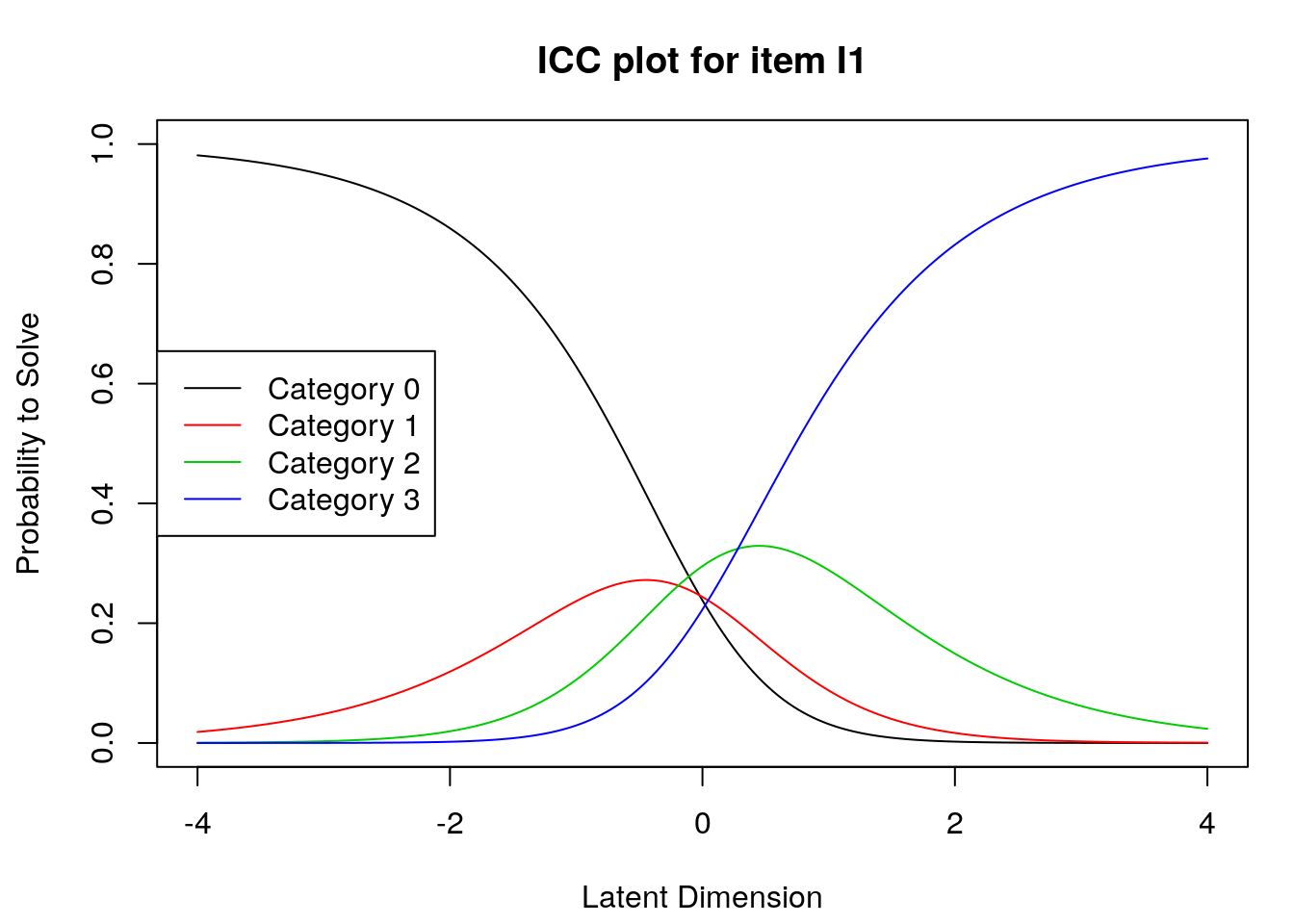
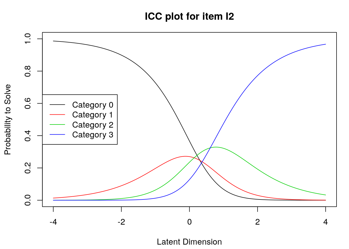
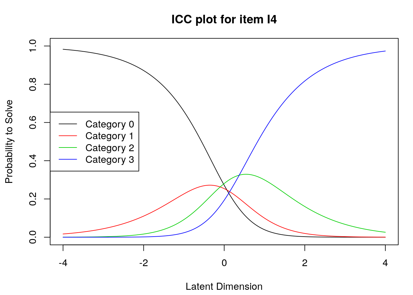
5.3.6 Graphic Information
5.3.6.1 Plot the Person-Item Map
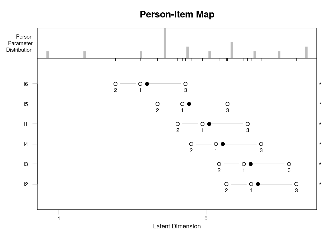
In this plot, we should consider the degree to which there is evidence of overlap between item and person locations (targeting).
We can also examine the individual items’ ordering on the logit scale with reference to our theory about the expected ordering.
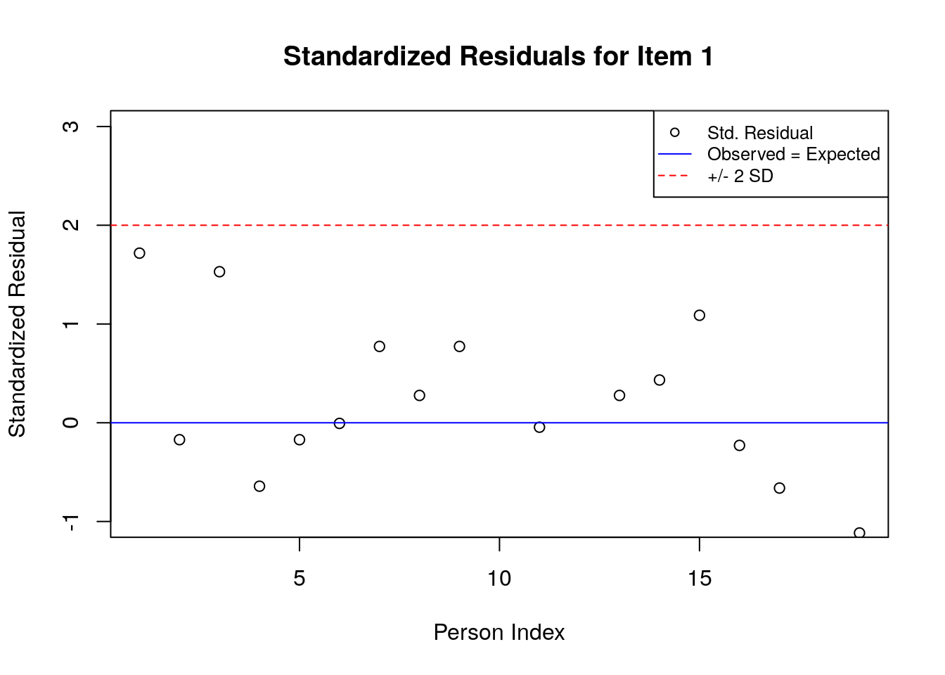
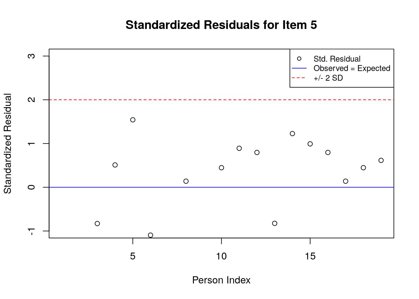
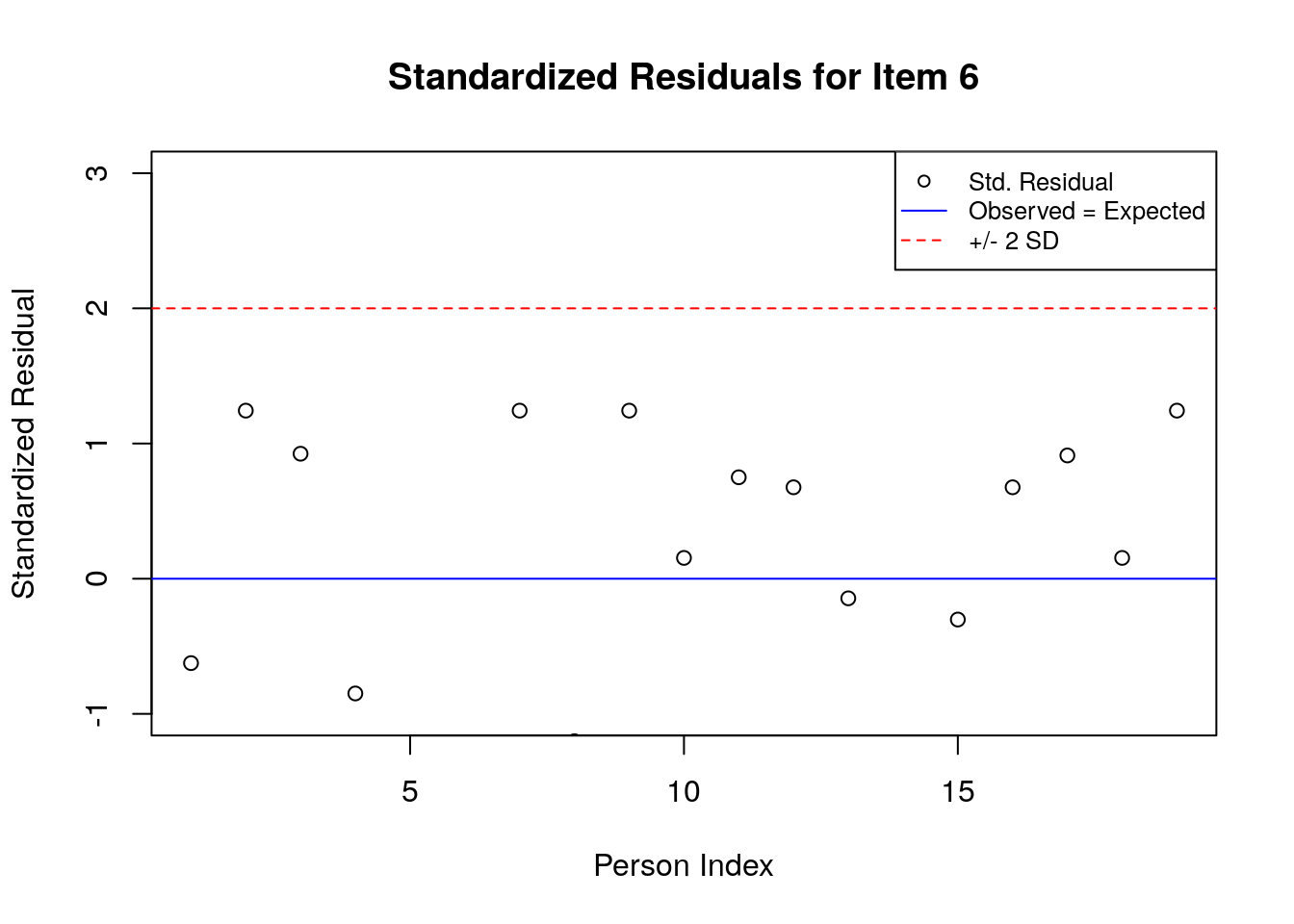
5.3.6.2 Plot the Standardized Residuals
stresid <- item.fit$st.res

# before constructing the plots, find the max & min residuals:
max.resid <- ceiling(max(stresid))
min.resid <- ceiling(min(stresid))

for(item.number in 1:ncol(stresid)){
  plot(stresid[, item.number], ylim = c(min.resid, max.resid),
       main = paste("Standardized Residuals for Item ", item.number, sep = ""),
       ylab = "Standardized Residual", xlab = "Person Index")
  abline(h = 0, col = "blue")
  abline(h=2, lty = 2, col = "red")
  abline(h=-2, lty = 2, col = "red")
  legend("topright", c("Std. Residual", "Observed = Expected", "+/- 2 SD"), pch = c(1, NA, NA),
         lty = c(NA, 1, 2),
         col = c("black", "blue", "red"), cex = .8)
}


5.4 Supplmentary Learning Materials
Andrich, D(1978). “A rating formulation for ordered response categories.” Psychometrika, 43(4), 561–573. doi:10.1007/BF02293814.
Mair, P., Hatzinger, R., & Maier M. J. (2020). eRm: Extended Rasch Modeling. 1.0-1. https://cran.r-project.org/package=eRm