Chapter 8 Basics of Differential Item Functioning
8.1 Purpose
The purpose of this lab is to introduce students to some basic differential item functioning (DIF) analyses based on Rasch models. We will use the “eRm” package for most of the analyses in this lab.
8.2 R-lab 1: DIF Analysis with the Dichotomous Rasch Model
8.2.1 Prepare the R-package and data set
# Load the package
library(eRm)
# If you want to cite the R packages that you're planning to use in your research article, you can use the citation function:
citation("eRm")
##
## To cite package 'eRm' in publications use:
##
## ###############################################################################
## The current Package Version:
##
## Mair, P., Hatzinger, R., & Maier M. J. (2020). eRm: Extended Rasch
## Modeling. 1.0-1. https://cran.r-project.org/package=eRm
##
## ###############################################################################
## The original JSS Article:
##
## Mair, P., & Hatzinger, R. (2007). Extended Rasch modeling: The eRm
## package for the application of IRT models in R. Journal of
## Statistical Software, 20(9), 1-20. http://www.jstatsoft.org/v20/i09
##
## ###############################################################################
## Article about CML Estimation in eRm:
##
## Mair, P., & Hatzinger, R. (2007). CML based estimation of extended
## Rasch models with the eRm package in R. Psychology Science, 49(1),
## 26-43.
##
## ###############################################################################
## Article about LLRAs in eRm:
##
## Hatzinger, R., & Rusch, T. (2009). IRT models with relaxed
## assumptions in eRm: A manual-like instruction. Psychology Science
## Quarterly, 51(1), 87-120.
##
## ###############################################################################
## Book Chapter about LLRAs:
##
## Rusch T., Maier M. J., & Hatzinger R. (2013). Linear logistic models
## with relaxed assumptions in R. In: B. Lausen, D. van den Poel, & A.
## Ultsch (Eds.) Algorithms from and for Nature and Life.New York:
## Springer. 337-347. http://dx.doi.org/10.1007/978-3-319-00035-0_34
##
## ###############################################################################
## Article about the performance of Quasi-Exact Tests in eRm:
##
## Koller, I., Maier, M. J., & Hatzinger, R. (2015). An Empirical Power
## Analysis of Quasi-Exact Tests for the Rasch Model: Measurement
## Invariance in Small Samples. Methodology, 11(2), 45-54.
## http://dx.doi.org/10.1027/1614-2241/a000090
##
## ###############################################################################
## Article about the Performance of the nonparametric Q3 Tests in eRm:
##
## Debelak, R., & Koller, I. (2019). Testing the Local Independence
## Assumption of the Rasch Model With Q3-Based Nonparametric Model
## Tests. Applied Psychological Measurement
## https://doi.org/10.1177/0146621619835501
##
## To see these entries in BibTeX format, use 'print(<citation>,
## bibtex=TRUE)', 'toBibtex(.)', or set
## 'options(citation.bibtex.max=999)'.Now, let’s load the data. We will practice running some DIF analyses based on the dichotomous Rasch model. To do this, we will use the “raschdat1” data that are provided as part of the “eRm” package.
##        I1             I2             I3             I4             I5
##  Min.   :0.00   Min.   :0.00   Min.   :0.00   Min.   :0.00   Min.   :0.00
##  1st Qu.:1.00   1st Qu.:0.00   1st Qu.:0.00   1st Qu.:0.00   1st Qu.:0.00
##  Median :1.00   Median :0.00   Median :1.00   Median :0.00   Median :0.00
##  Mean   :0.76   Mean   :0.47   Mean   :0.62   Mean   :0.33   Mean   :0.22
##  3rd Qu.:1.00   3rd Qu.:1.00   3rd Qu.:1.00   3rd Qu.:1.00   3rd Qu.:0.00
##  Max.   :1.00   Max.   :1.00   Max.   :1.00   Max.   :1.00   Max.   :1.00
##        I6             I7            I8             I9            I10
##  Min.   :0.00   Min.   :0.0   Min.   :0.00   Min.   :0.00   Min.   :0.00
##  1st Qu.:0.00   1st Qu.:0.0   1st Qu.:0.00   1st Qu.:0.00   1st Qu.:0.00
##  Median :0.00   Median :1.0   Median :1.00   Median :1.00   Median :0.00
##  Mean   :0.48   Mean   :0.6   Mean   :0.61   Mean   :0.57   Mean   :0.25
##  3rd Qu.:1.00   3rd Qu.:1.0   3rd Qu.:1.00   3rd Qu.:1.00   3rd Qu.:0.25
##  Max.   :1.00   Max.   :1.0   Max.   :1.00   Max.   :1.00   Max.   :1.00
##       I11            I12            I13            I14            I15
##  Min.   :0.00   Min.   :0.00   Min.   :0.00   Min.   :0.00   Min.   :0.00
##  1st Qu.:0.00   1st Qu.:0.00   1st Qu.:0.00   1st Qu.:0.00   1st Qu.:0.00
##  Median :0.00   Median :1.00   Median :0.00   Median :0.00   Median :1.00
##  Mean   :0.33   Mean   :0.54   Mean   :0.19   Mean   :0.12   Mean   :0.53
##  3rd Qu.:1.00   3rd Qu.:1.00   3rd Qu.:0.00   3rd Qu.:0.00   3rd Qu.:1.00
##  Max.   :1.00   Max.   :1.00   Max.   :1.00   Max.   :1.00   Max.   :1.00
##       I16            I17            I18            I19            I20
##  Min.   :0.00   Min.   :0.00   Min.   :0.00   Min.   :0.00   Min.   :0.0
##  1st Qu.:0.00   1st Qu.:0.00   1st Qu.:0.00   1st Qu.:0.00   1st Qu.:0.0
##  Median :0.00   Median :1.00   Median :0.00   Median :0.00   Median :1.0
##  Mean   :0.34   Mean   :0.53   Mean   :0.44   Mean   :0.31   Mean   :0.6
##  3rd Qu.:1.00   3rd Qu.:1.00   3rd Qu.:1.00   3rd Qu.:1.00   3rd Qu.:1.0
##  Max.   :1.00   Max.   :1.00   Max.   :1.00   Max.   :1.00   Max.   :1.0
##       I21            I22            I23           I24            I25
##  Min.   :0.00   Min.   :0.00   Min.   :0.0   Min.   :0.00   Min.   :0.0
##  1st Qu.:0.00   1st Qu.:0.00   1st Qu.:0.0   1st Qu.:0.00   1st Qu.:0.0
##  Median :1.00   Median :1.00   Median :1.0   Median :0.00   Median :0.0
##  Mean   :0.65   Mean   :0.66   Mean   :0.6   Mean   :0.46   Mean   :0.3
##  3rd Qu.:1.00   3rd Qu.:1.00   3rd Qu.:1.0   3rd Qu.:1.00   3rd Qu.:1.0
##  Max.   :1.00   Max.   :1.00   Max.   :1.0   Max.   :1.00   Max.   :1.0
##       I26           I27            I28           I29            I30
##  Min.   :0.0   Min.   :0.00   Min.   :0.0   Min.   :0.00   Min.   :0.00
##  1st Qu.:0.0   1st Qu.:0.00   1st Qu.:0.0   1st Qu.:0.00   1st Qu.:0.00
##  Median :1.0   Median :0.00   Median :0.0   Median :0.00   Median :1.00
##  Mean   :0.7   Mean   :0.44   Mean   :0.4   Mean   :0.31   Mean   :0.61
##  3rd Qu.:1.0   3rd Qu.:1.00   3rd Qu.:1.0   3rd Qu.:1.00   3rd Qu.:1.00
##  Max.   :1.0   Max.   :1.00   Max.   :1.0   Max.   :1.00   Max.   :1.00
8.2.2 Run dichotomous Rasch model
### Analyze the data using the dichotomous Rasch model:
dichot_model <- RM(raschdat1)
summary(dichot_model)
##
## Results of RM estimation:
##
## Call: RM(X = raschdat1)
##
## Conditional log-likelihood: -1434.482
## Number of iterations: 28
## Number of parameters: 29
##
## Item (Category) Difficulty Parameters (eta): with 0.95 CI:
## Estimate Std. Error lower CI upper CI
## I2 -0.051 0.216 -0.475 0.373
## I3 -0.782 0.222 -1.217 -0.347
## I4 0.650 0.228 0.204 1.096
## I5 1.301 0.254 0.802 1.799
## I6 -0.099 0.216 -0.523 0.324
## I7 -0.682 0.220 -1.113 -0.250
## I8 -0.732 0.221 -1.165 -0.299
## I9 -0.534 0.218 -0.961 -0.106
## I10 1.108 0.245 0.628 1.587
## I11 0.650 0.228 0.204 1.096
## I12 -0.388 0.217 -0.813 0.037
## I13 1.511 0.267 0.988 2.034
## I14 2.116 0.316 1.497 2.735
## I15 -0.340 0.216 -0.764 0.085
## I16 0.597 0.226 0.154 1.041
## I17 -0.340 0.216 -0.764 0.085
## I18 0.094 0.217 -0.332 0.520
## I19 0.759 0.231 0.306 1.211
## I20 -0.682 0.220 -1.113 -0.250
## I21 -0.937 0.226 -1.379 -0.495
## I22 -0.989 0.227 -1.434 -0.544
## I23 -0.682 0.220 -1.113 -0.250
## I24 -0.003 0.217 -0.427 0.422
## I25 0.814 0.233 0.358 1.271
## I26 -1.207 0.234 -1.665 -0.749
## I27 0.094 0.217 -0.332 0.520
## I28 0.290 0.220 -0.140 0.721
## I29 0.759 0.231 0.306 1.211
## I30 -0.732 0.221 -1.165 -0.299
##
## Item Easiness Parameters (beta) with 0.95 CI:
## Estimate Std. Error lower CI upper CI
## beta I1 1.565 0.249 1.077 2.053
## beta I2 0.051 0.216 -0.373 0.475
## beta I3 0.782 0.222 0.347 1.217
## beta I4 -0.650 0.228 -1.096 -0.204
## beta I5 -1.301 0.254 -1.799 -0.802
## beta I6 0.099 0.216 -0.324 0.523
## beta I7 0.682 0.220 0.250 1.113
## beta I8 0.732 0.221 0.299 1.165
## beta I9 0.534 0.218 0.106 0.961
## beta I10 -1.108 0.245 -1.587 -0.628
## beta I11 -0.650 0.228 -1.096 -0.204
## beta I12 0.388 0.217 -0.037 0.813
## beta I13 -1.511 0.267 -2.034 -0.988
## beta I14 -2.116 0.316 -2.735 -1.497
## beta I15 0.340 0.216 -0.085 0.764
## beta I16 -0.597 0.226 -1.041 -0.154
## beta I17 0.340 0.216 -0.085 0.764
## beta I18 -0.094 0.217 -0.520 0.332
## beta I19 -0.759 0.231 -1.211 -0.306
## beta I20 0.682 0.220 0.250 1.113
## beta I21 0.937 0.226 0.495 1.379
## beta I22 0.989 0.227 0.544 1.434
## beta I23 0.682 0.220 0.250 1.113
## beta I24 0.003 0.217 -0.422 0.427
## beta I25 -0.814 0.233 -1.271 -0.358
## beta I26 1.207 0.234 0.749 1.665
## beta I27 -0.094 0.217 -0.520 0.332
## beta I28 -0.290 0.220 -0.721 0.140
## beta I29 -0.759 0.231 -1.211 -0.306
## beta I30 0.732 0.221 0.299 1.1658.2.3 Identify subgroups
Then,we need to identify the subgroups between which you will examine DIF. Since our data are made up, so we will make up subgroup classifications as well. We will do this by sampling 100 observations with replacement from a vector made up of the numbers “1” and “2” to match our 100-person data.
Then we will calculate subgroup-specific item difficulty values using the Waldtest() function from “eRm”.
# Calculate subgroup-specific item difficulty values:
subgroup_diffs <- Waldtest(dichot_model, splitcr = subgroups)
This analysis saves numerous details to the object called “subgroup_diffs”. Let’s create new objects with the group-specific item difficulties:
# Create objects for subgroup-specific item difficulties:
subgroup_1_diffs <- subgroup_diffs$betapar1
subgroup_2_diffs <- subgroup_diffs$betapar2
8.2.3.1 Examine test-statistic result for the item comparisons
First, let’s examine the test statistics & p-values for the item comparisons. Let’s create an object called “comparisons” in which we store the results:
#store results from item comparisons in an object called "comparisons"
comparisons <- as.data.frame(subgroup_diffs$coef.table)
You can view the “comparisons” object by clicking on it in your Environment pane in the upper right corner of R Studio.
Once you click on “comparisons” you will see a preview of the comparison results.
Sorting the results by p-value by clicking the arrow in the top right corner of the “p-value” column until the values are sorted from low to high.
From these results, we see that there is one item with a statistically significant difference based on p < 0.05; Item 20 and Item 8.
8.2.4 Visualize the test statistics for the item comparison
It is often useful to visualize the test statistics for the item comparison. You can do this using a simple scatterplot. Ti. To run the scatterplot code all at once, highlight/select the code between “#start” and “# stop” and run it.
graphics.off()
min.y <- ifelse(ceiling(min(comparisons$`z-statistic`)) > -3, -3,
                ceiling(min(comparisons$`z-statistic`)))

max.y <- ifelse(ceiling(max(comparisons$`z-statistic`)) < 3, 3,
                ceiling(max(comparisons$`z-statistic`)))

plot(comparisons$`z-statistic`, ylim = c(min.y, max.y),
     ylab = "Z", xlab = "Item", main = "Test Statistics for Item Comparisons \nbetween Subgroup 1 and Subgroup 2")
abline(h=2, col = "red", lty = 2)
abline(h=-2, col = "red", lty = 2)

legend("topright", c("Z Statistic", "Boundaries for Significant Difference"),
       pch = c(1, NA), lty = c(NA, 2), col = c("black", "red"), cex = .7)
This plot highlights items that are significantly different between subgroups.
8.2.5 Export the item comparison results for later use using the following code.
# Take out the values that we need for our comparison table
comparison.results <- cbind.data.frame(c(1:length(subgroup_1_diffs)),
                                       subgroup_1_diffs, subgroup_diffs$se.beta1,
                                       subgroup_2_diffs, subgroup_diffs$se.beta2,
                                       comparisons)
# Name the columns of the results
names(comparison.results) <- c("Item",
                             "Subgroup_1_Difficulty", "Subgroup_1_SE",
                               "Subgroup_2_Difficulty", "Subgroup_2_SE",
                               "Z", "p_value")
# Put the result into a csv file
write.csv(comparison.results, file = "comparison_results.csv")
8.2.6 Plot the item difference
Now, let’s make a scatterplot of the item differences for the two subgroups.
NOTE: Because the procedure that we used to calculate item difficulties specific to each subgroup has already adjusted the difficulties to be on the same scale, we don’t need to apply any transformation.
The following code will create a scatterplot with 95% confidence bands to highlight items that are significantly different between the subgroups.
### DIF Scatterplots:

## First, calculate values for constructing the confidence bands:

mean.1.2 <- ((subgroup_1_diffs - mean(subgroup_1_diffs))/2*sd(subgroup_1_diffs) +
               (subgroup_2_diffs - mean(subgroup_2_diffs))/2*sd(subgroup_2_diffs))

joint.se <- sqrt((subgroup_diffs$se.beta1^2/sd(subgroup_1_diffs)) +
                   (subgroup_diffs$se.beta2^2/sd(subgroup_2_diffs)))


upper.group.1 <- mean(subgroup_1_diffs) + ((mean.1.2 - joint.se )*sd(subgroup_1_diffs))
upper.group.2 <- mean(subgroup_2_diffs) + ((mean.1.2 + joint.se )*sd(subgroup_2_diffs))

lower.group.1 <- mean(subgroup_1_diffs) + ((mean.1.2 + joint.se )*sd(subgroup_1_diffs))
lower.group.2 <- mean(subgroup_2_diffs) + ((mean.1.2 - joint.se )*sd(subgroup_2_diffs))


upper <- cbind.data.frame(upper.group.1, upper.group.2)
upper <- upper[order(upper$upper.group.1, decreasing = FALSE),]


lower <- cbind.data.frame(lower.group.1, lower.group.2)
lower <- lower[order(lower$lower.group.1, decreasing = FALSE),]

## make the scatterplot:

plot(subgroup_1_diffs, subgroup_2_diffs, xlim = c(-2, 2), ylim = c(-2, 2),
     xlab = "Group 1", ylab = "Group 2", main = "Group 1 Measures \n plotted against \n Group 2 Measures")
abline(a = 0, b = 1, col = "purple")

par(new = T)

lines(upper$upper.group.1, upper$upper.group.2, lty = 2, col = "red")

lines(lower$lower.group.1, lower$lower.group.2, lty = 2, col = "red")

legend("bottomright", c("Item Location", "Identity Line", "95% Confidence Band"),
       pch = c(1, NA, NA), lty = c(NA, 1, 2), col = c("black", "purple", "red"))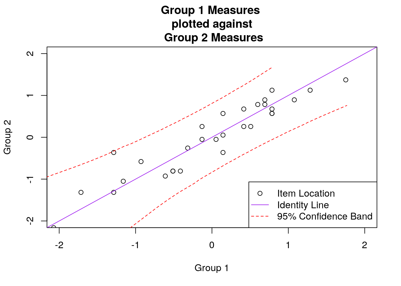
Finally, let’s make a bar plot to illustrate the differences in item difficulty between the subgroups.
### Bar plot of item differences:

# First, calculate difference in difficulty between subgroups
# Note that I multiplied by -1 to reflect item difficulty rather than easiness (eRm quirk):
item_dif <- (subgroup_1_diffs*-1)-(subgroup_2_diffs*-1)


# Code to use different colors to highlight items with differences >= .5 logits:
colors <- NULL

for (item.number in 1:30){

  colors[item.number] <- ifelse(abs(item_dif[item.number]) > .5, "dark blue", "light green")

}

# Bar plot code:
item_dif <- as.vector(item_dif)

x <- barplot(item_dif, horiz = TRUE, xlim = c(-2, 2),
             col = colors,
             ylim = c(1,40),
             xlab = "Logit Difference")

# code to add labels to the plot:

dif_labs <- NULL

for (i in 1:length(subgroup_1_diffs)) {
  dif_labs[i] <- ifelse(item_dif[i] < 0, item_dif[i] - .2,
                        item_dif[i] + .2)
}

text(dif_labs, x, labels = c(1:length(subgroup_1_diffs)),
     xlim = c(-1.5, 1.5), cex = .8)

# add vertical lines to highlight .5 logit differences:
abline(v = .5, lty = 3)
abline(v = -.5, lty = 3)

# add additional text to help with interpretation:

text(-1, 40, "Easier to Endorse for Group 1", cex = .8)
text(1, 40, "Easier to Endorse for Group 2", cex = .8)

legend("bottomright", c("Diff >= .5 logits", "Diff < .5 logits"),
       pch = 15, col = c("dark blue", "light green"), cex = .7 )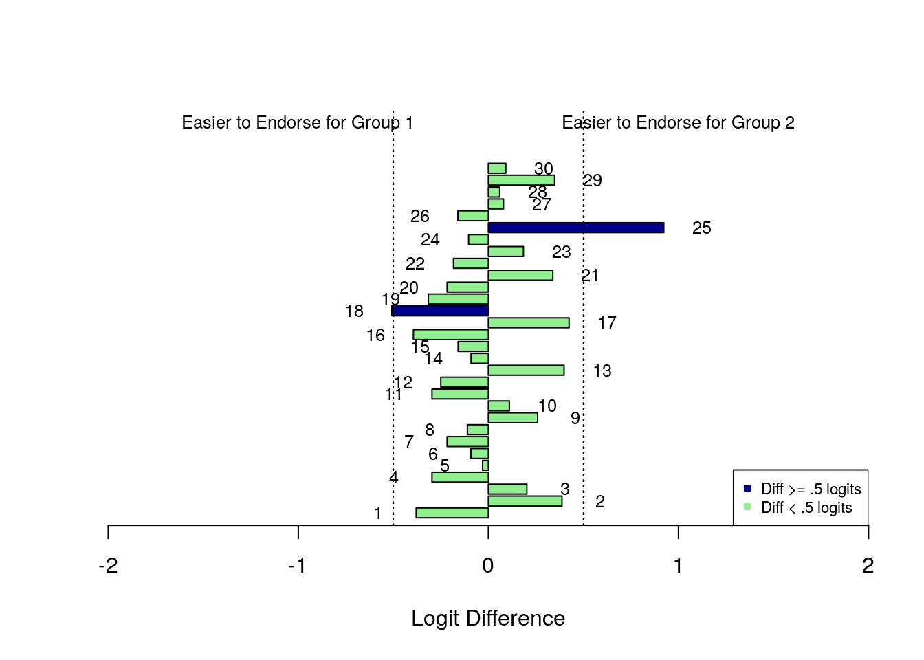
8.3 R-lab 2: DIF Analysis with the Partial Credit Model
We will practice running some DIF analyses based on the Partial Credit model. To do this, we will use the “pcmdat2” data that are provided as part of the eRm package. Most of the procedures for this analysis mirror those from Part One. As a result, less detail will be provided in this part of the lab except where needed to highlight differences.
8.3.1 Load the data into your working environment and generate a summary of responses
##        I1              I2               I3              I4
##  Min.   :0.000   Min.   :0.0000   Min.   :0.000   Min.   :0.00
##  1st Qu.:0.000   1st Qu.:0.0000   1st Qu.:1.000   1st Qu.:1.00
##  Median :1.000   Median :1.0000   Median :2.000   Median :1.00
##  Mean   :1.013   Mean   :0.9067   Mean   :1.527   Mean   :1.38
##  3rd Qu.:2.000   3rd Qu.:2.0000   3rd Qu.:2.000   3rd Qu.:2.00
##  Max.   :2.000   Max.   :2.0000   Max.   :2.000   Max.   :2.00
8.3.2 Run the Partial Credit Model
Analyze the data using the Partial Credit model, and store the results in an object called “PC_model”
8.3.3 Conduct DIF analyses
NOTE! The estimation procedure for polytomous (> 2 categories) data procedures estimates of rating scale category thresholds for each item. If you want to compare the threshold locations between subgroups, you can use: subgroup_diffs <- Waldtest(PC_model, splitcr = subgroups) to generate the DIF results specific to item-category thresholds, and then proceed as in Part two.
However, if you want to make comparisons at the overall item level, you’ll need to get item difficulty estimates and standard errors for the overall item. You can do this using the following code.
### DIF analysis

# Create subgroup classifications:
subgroups <- rep(c(1,2), nrow(pcmdat2)/2)

# Calculate subgroup-specific item difficulty values (#select/highlight code starting here):

#- First, get overall item difficulties specific to each subgroup:

group1_item.diffs.overall <- NULL
group2_item.diffs.overall <- NULL

responses <- pcmdat2 # update this if needed with the responses object
model.results <- PC_model # update this if needed with the model results object

responses.g <- cbind.data.frame(subgroups, responses)
responses.g1 <- subset(responses.g, responses.g$subgroups == 1)
responses.g2 <- subset(responses.g, responses.g$subgroups == 2)

## Compare thresholds between groups:
subgroup_diffs <- Waldtest(PC_model, splitcr = subgroups)


for(item.number in 1:ncol(responses)){

  n.thresholds.g1 <-  length(table(responses.g1[, item.number+1]))-1

  group1_item.diffs.overall[item.number] <- mean(subgroup_diffs$betapar1[((item.number*(n.thresholds.g1))-(n.thresholds.g1-1)):
                                                                           (item.number*(n.thresholds.g1))])*-1

  n.thresholds.g2 <-  length(table(responses.g2[, item.number+1]))-1

  group2_item.diffs.overall[item.number] <- mean(subgroup_diffs$betapar2[((item.number*(n.thresholds.g2))-(n.thresholds.g2-1)):
                                                                           (item.number*(n.thresholds.g2))])*-1
}

group1_item.diffs.overall
## [1] 1.0190150 1.8180476 -2.2656087 -0.5714538## [1] 0.9498830 1.3407300 -1.7819067 -0.5087063## Get overall item SE values:
#- First, get overall SEs specific to each subgroup:
group1_item.se.overall <- NULL
group2_item.se.overall <- NULL
responses <- pcmdat2 # update this if needed with the responses object
model.results <- PC_model # update this if needed with the model results object
responses.g <- cbind.data.frame(subgroups, responses)
responses.g1 <- subset(responses.g, responses.g$subgroups == 1)
responses.g2 <- subset(responses.g, responses.g$subgroups == 2)
subgroup_diffs <- Waldtest(PC_model, splitcr = subgroups)
for(item.number in 1:ncol(responses)){
n.thresholds.g1 <- length(table(responses.g1[, item.number+1]))-1
group1_item.se.overall[item.number] <- mean(subgroup_diffs$se.beta1[((item.number*(n.thresholds.g1))-(n.thresholds.g1-1)):
(item.number*(n.thresholds.g1))])
n.thresholds.g2 <- length(table(responses.g2[, item.number+1]))-1
group2_item.se.overall[item.number] <- mean(subgroup_diffs$se.beta2[((item.number*(n.thresholds.g2))-(n.thresholds.g2-1)):
(item.number*(n.thresholds.g2))])
}
group1_item.se.overall## [1] 0.2787479 0.2874604 0.4721574 0.3033779## [1] 0.2666859 0.2613309 0.4142456 0.2922317Then, we will use our own code to calculate test statistics for the differences in overall item difficulties:
# Calculate test statistics for item comparisons:
z <- (group1_item.diffs.overall - group2_item.diffs.overall)/
sqrt(group1_item.se.overall^2 + group2_item.se.overall^2)

# view test statistics in the console:
z
## [1] 0.1792031 1.2286368 -0.7700816 -0.14896158.3.4 Make a scatterplot
# Plot the test statistics:
min.y <- ifelse(ceiling(min(z)) > -3, -3,
                ceiling(min(z)))

max.y <- ifelse(ceiling(max(z)) < 3, 3,
                ceiling(max(z)))

plot(z, ylim = c(min.y, max.y),
     ylab = "Z", xlab = "Item", main = "Test Statistics for Item Comparisons \nbetween Subgroup 1 and Subgroup 2",
     axes=FALSE)
axis(1, at = c(1, 2, 3, 4), labels = c(1, 2, 3, 4))
axis(2)
abline(h=2, col = "red", lty = 2)
abline(h=-2, col = "red", lty = 2)

legend("topright", c("Z Statistic", "Boundaries for Significant Difference"),
       pch = c(1, NA), lty = c(NA, 2), col = c("black", "red"), cex = .7)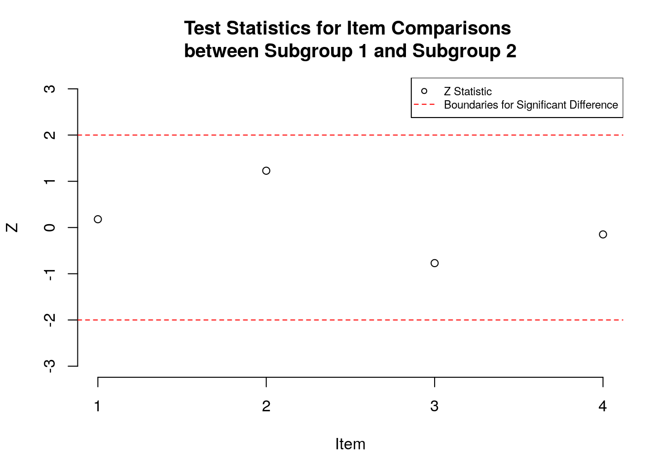
Export item comparison results to a .csv file
# Export item comparison results:

comparison.results <- cbind.data.frame(c(1:length(group1_item.diffs.overall)),
                                       group1_item.diffs.overall, group1_item.se.overall,
                                       group2_item.diffs.overall, group2_item.se.overall,
                                       z)

names(comparison.results) <- c("Item",
                               "Subgroup_1_Difficulty", "Subgroup_1_SE",
                               "Subgroup_2_Difficulty", "Subgroup_2_SE",
                               "Z")

comparison.results <- round(comparison.results, digits = 2)
write.csv(comparison.results, file = "PCM_comparison_results.csv", row.names = FALSE)
8.3.5 Create scatterplot of item measures
Create scatterplot of item measures with 95% confidence bands
### DIF Scatterplot:

## First, calculate values for constructing the confidence bands:

mean.1.2 <- ((group1_item.diffs.overall - mean(group1_item.diffs.overall))/2*sd(group1_item.diffs.overall) +
               (group2_item.diffs.overall - mean(group2_item.diffs.overall))/2*sd(group2_item.diffs.overall))

joint.se <- sqrt((group1_item.se.overall^2/sd(group1_item.diffs.overall)) +
                   (group2_item.se.overall^2/sd(group2_item.diffs.overall)))


upper.group.1 <- mean(group1_item.diffs.overall) + ((mean.1.2 - joint.se )*sd(group1_item.diffs.overall))
upper.group.2 <- mean(group2_item.diffs.overall) + ((mean.1.2 + joint.se )*sd(group2_item.diffs.overall))

lower.group.1 <- mean(group1_item.diffs.overall) + ((mean.1.2 + joint.se )*sd(group1_item.diffs.overall))
lower.group.2 <- mean(group2_item.diffs.overall) + ((mean.1.2 - joint.se )*sd(group1_item.diffs.overall))


upper <- cbind.data.frame(upper.group.1, upper.group.2)
upper <- upper[order(upper$upper.group.1, decreasing = FALSE),]


lower <- cbind.data.frame(lower.group.1, lower.group.2)
lower <- lower[order(lower$lower.group.1, decreasing = FALSE),]

## make the scatterplot:

plot(group1_item.diffs.overall, group2_item.diffs.overall, xlim = c(-3, 3), ylim = c(-3, 3),
     xlab = "Group 1", ylab = "Group 2", main = "Group 1 Measures \n plotted against \n Group 2 Measures")
abline(a = 0, b = 1, col = "purple")

par(new = T)

lines(upper$upper.group.1, upper$upper.group.2, lty = 2, col = "red")

lines(lower$lower.group.1, lower$lower.group.2, lty = 2, col = "red")

legend("bottomright", c("Item Location", "Identity Line", "95% Confidence Band"),
       pch = c(1, NA, NA), lty = c(NA, 1, 2), col = c("black", "purple", "red"))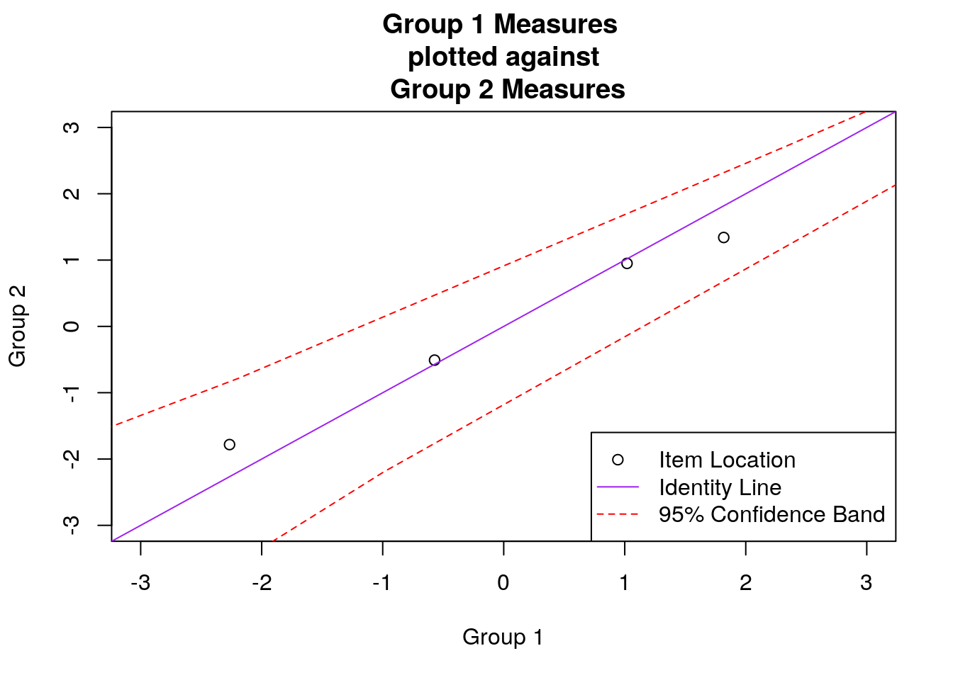
8.3.6 Create bar plot of item differences
### Bar plot of item differences:

# First, calculate difference in difficulty between subgroups
item_dif <- group1_item.diffs.overall - group2_item.diffs.overall

# Code to use different colors to highlight items with differences >= .5 logits:
colors <- NULL

for (item.number in 1:ncol(responses)){
  colors[item.number] <- ifelse(abs(item_dif[item.number]) > .5, "dark blue", "light green")
}

# Bar plot code:
item_dif <- as.vector(item_dif)

x <- barplot(item_dif, horiz = TRUE, xlim = c(-2, 2),
             col = colors,
             #=ylim = c(1,4),
             xlab = "Logit Difference")

# code to add labels to the plot:

dif_labs <- NULL

for (i in 1:length(group1_item.diffs.overall)) {
  dif_labs[i] <- ifelse(item_dif[i] < 0, item_dif[i] - .2,
                        item_dif[i] + .2)
}

text(dif_labs, x, labels = c(1:length(group1_item.diffs.overall)),
     xlim = c(-1.5, 1.5), cex = .8)

# add vertical lines to highlight .5 logit differences:
abline(v = .5, lty = 3)
abline(v = -.5, lty = 3)

# add additional text to help with interpretation:

text(-1, 4.5, "Easier to Endorse for Group 1", cex = .8)
text(1, 4.5, "Easier to Endorse for Group 2", cex = .8)

legend("bottomright", c("Diff >= .5 logits", "Diff < .5 logits"),
       pch = 15, col = c("dark blue", "light green"), cex = .7 )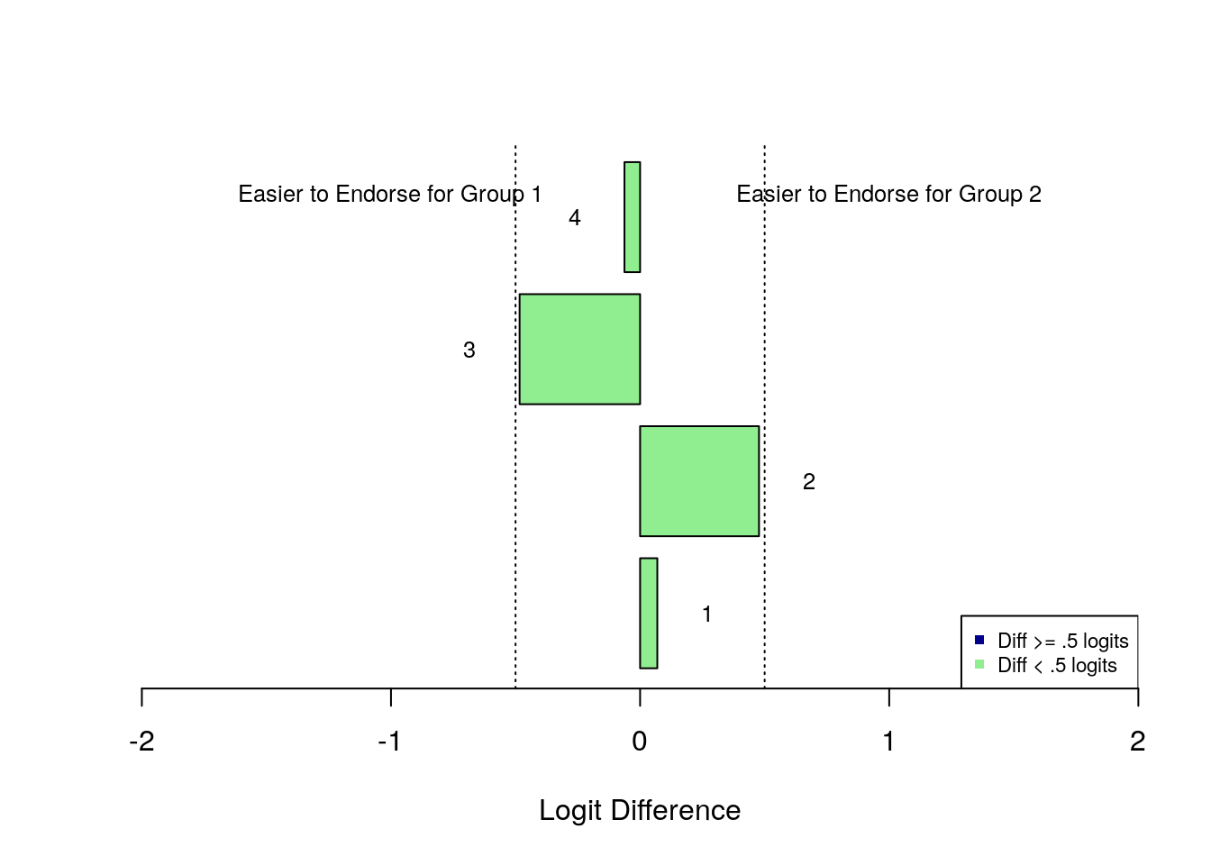
8.4 Example APA-format results section for basic DIF analysis
In this analysis, we examined the degree to which there was evidence of uniform differential item functioning (DIF) between two subgroups of participants (group 1 and group 2) in the “pcmdat2” example dataset from the using the Extended Rasch Models (“eRm”) package (Mair, Hatzinger, & Maier, 2020) for R. The data included 300 participants’ responses to four rating scale items made up of three ordered categories (X = 0, 1, or 2). We used the eRm package to conduct all of the analyses.
As a first step in the analysis, we examined item difficulty estimates and standard errors specific to each subgroup using the Partial Credit model (Masters, 1982). We estimated item difficulty for the two subgroups using a combined analysis of both subgroups and then estimating the group-specific item difficulties using the eRm package. Group-specific item difficulties and standard errors are shown in Table 1.
To examine the differences in item difficulty between subgroups, we calculated standardized differences following Wright and Masters (1982) as follows: \[z=\left(d_{1}-d_{2}\right) / \sqrt{se_{1}^{2}+se_{2}^{2}}\]
where \(z\) is the standardized difference, d1 is the item difficulty specific to Subgroup 1, d2 is the item difficulty specific to Subgroup 2, \(se_{1}^{2}\) is the standard error of the item difficulty specific to Subgroup 1, and \(se_{2}^{2}\) is the standard error of the item difficulty specific to Subgroup 2. Using the formulation of the z statistic, higher values of z indicate higher item locations (more-difficult to endorse) for Subgroup 1 compared to Subgroup 2.
Figure 1 shows a plot of the z-statistics for the four survey items; these values are also presented numerically in Table 1. In the figure, the x-axis shows the item identification numbers, and the y-axis shows the value of the z-statistic. Boundaries at +2 and -2 are indicated using dashed horizontal lines to highlight statistically significant differences in item difficulty between subgroups. Examination of these results indicates that the items were not significantly different in difficulty between the two subgroups. In addition, there were both positive and negative z statistics, indicating that although the differences in item difficulty were not significant, there were some items that were easier to endorse for Subgroup 1 and others that were easier to endorse for Subgroup 2.
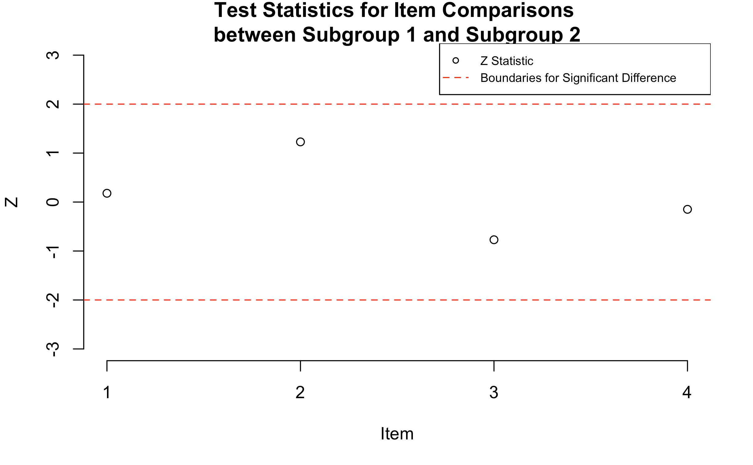
Figure 1: Plot of Standardized Differences for Items between Subgroups
To further explore the differences in item difficulty between the two subgroups, Figure 2 shows a scatterplot of the item locations between the two subgroups. In the plot, the item difficulty for Subgroup 1 is shown on the x-axis, and the item difficulty for Subgroup 2 is shown on the y-axis. Individual items are indicated using open circle plotting symbols. A solid identity line is included to highlight deviations from invariant item difficulties between the two groups: Points that fall below this line indicate that items were easier to endorse (lower item measures) for Subgroup 2, and points that fall above the line indicate that items were easier to endorse (lower item measures) for Subgroup 1. Dashed lines are also included to indicate a 95% confidence interval for the difference between the item measures, following Luppescu (1995).
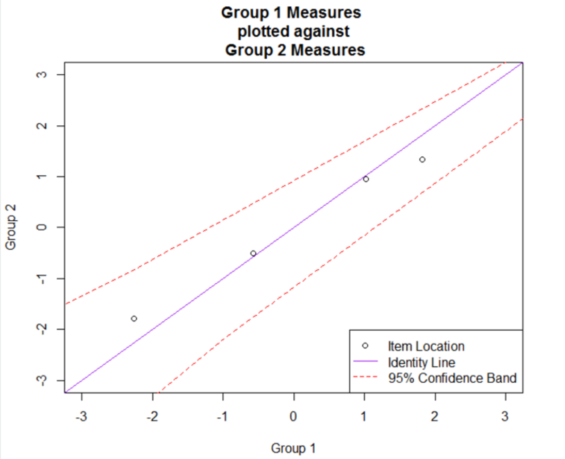
Figure 2: Scatterplot of Subgroup-Specific Item Difficulties
Finally, Figure 3 is a bar plot that illustrates the direction and magnitude of the differences in item difficulty between subgroups. In the plot, each bar represents the difference in difficulty between subgroups for an individual item, ordered by the item sequence in the survey. Bars that point to the left of the plot indicate that the item was easier to endorse for Subgroup 1, and bars that point to the right of the plot indicate that the item was easier to endorse for Subgroup 2. Dashed vertical lines are plotted that show values of +0.5 and -0.5 logits as an indicator of substantial differences in item difficulty between subgroups.
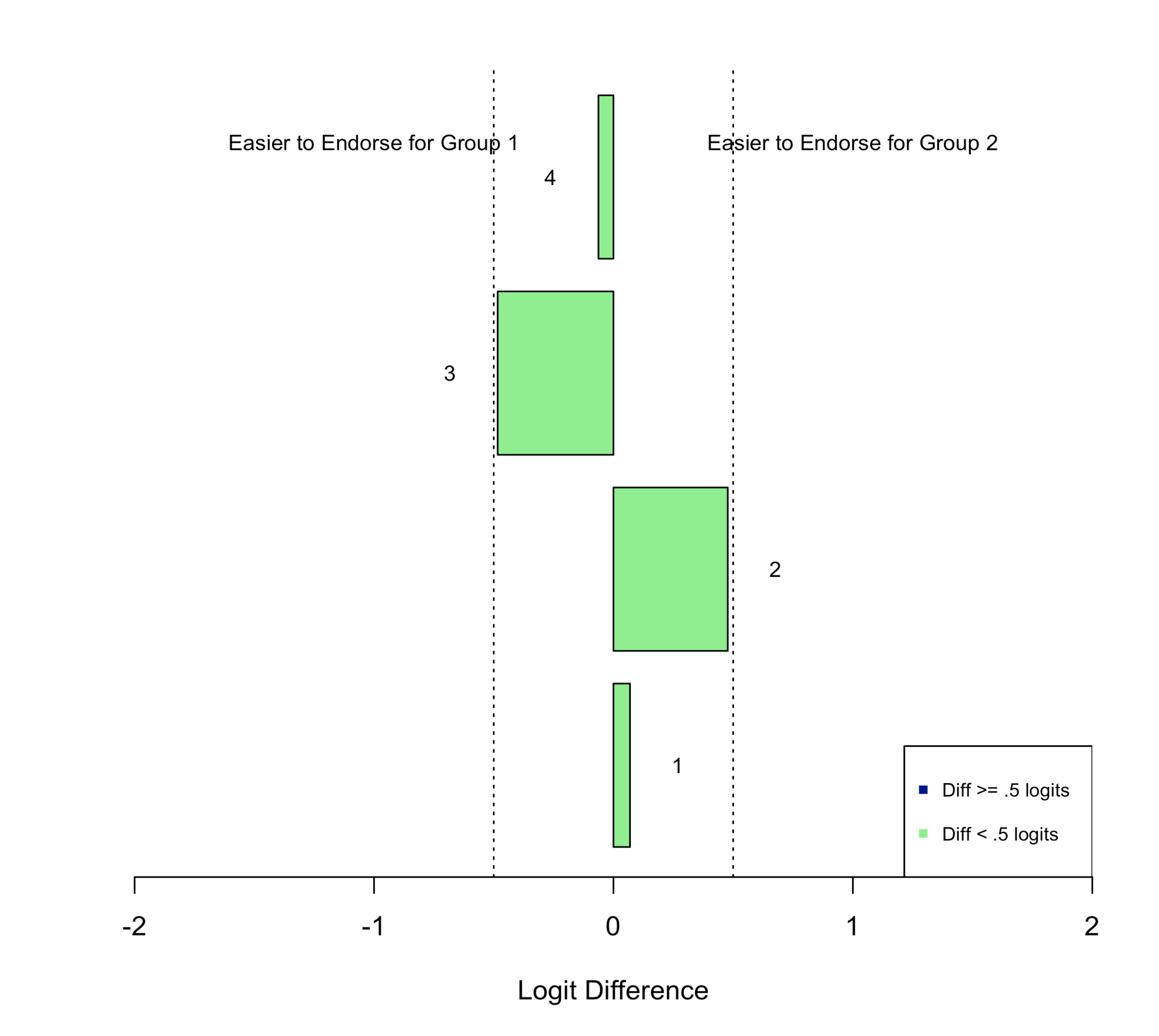
Figure 3: Bar Plot of Differences In Item Difficulty Between Subgroups
8.5 References
Luppescu, S. (1995). Comparing measures: Scatterplots. Rasch Measurement Transactions, 9(1), 410.
Masters, G. N. (1982). A Rasch model for partial credit scoring. Psychometrika, 47(2), 149–174. https://doi.org/10.1007/BF02296272
Masters, G. N., & Wright, B. D. (1997). The partial credit model. In W. J. van der Linden & R. K. Hambleton (Eds.), Handbook of modern item response theory (pp. 101–121). Springer.
Mair, P., Hatzinger, R., & Maier M. J. (2020). eRm: Extended Rasch Modeling. 1.0-1. https://cran.r-project.org/package=eRm
Wright, B. D., & Masters, G. N. (1982). Rating Scale Analysis: Rasch Measurement. MESA Press.