Chapter 9 Rating Scale Evaluation
9.1 R-lab purpose
The purpose of this lab is to give students experience running some basic rating scale analyses using Rasch models. From Blackboard, please download and save these files to a convenient location on your computer.
ratings.csv pain_cleaned_numeric.csv
We will use “eRm” package for this analysis.
9.2 R-lab: Rating Scale Analysis on Example Survey Data
For our first analysis, we will try conducting basic rating scale functioning analyses using some example survey data.
9.2.1 Load and investigate the data set
# load the example survey data into your working environment and generate a summary of the data
survey.responses <- read.csv("ratings.csv")
summary(survey.responses)
## id i1 i2 i3
## Min. : 1.00 Min. :0.00 Min. :0.000 Min. :0.000
## 1st Qu.: 88.25 1st Qu.:1.00 1st Qu.:1.000 1st Qu.:2.000
## Median :175.50 Median :2.00 Median :2.000 Median :3.000
## Mean :175.50 Mean :1.86 Mean :1.654 Mean :2.934
## 3rd Qu.:262.75 3rd Qu.:3.00 3rd Qu.:3.000 3rd Qu.:4.000
## Max. :350.00 Max. :4.00 Max. :4.000 Max. :4.000
## i4 i5 i6 i7
## Min. :0.000 Min. :0.000 Min. :0.000 Min. :0.000
## 1st Qu.:1.000 1st Qu.:1.000 1st Qu.:2.000 1st Qu.:1.000
## Median :2.000 Median :2.000 Median :3.000 Median :2.000
## Mean :1.937 Mean :2.114 Mean :2.543 Mean :2.046
## 3rd Qu.:3.000 3rd Qu.:3.000 3rd Qu.:3.000 3rd Qu.:3.000
## Max. :4.000 Max. :4.000 Max. :4.000 Max. :4.000
## i8 i9 i10 i11
## Min. :0.000 Min. :0.000 Min. :0.000 Min. :0.000
## 1st Qu.:2.000 1st Qu.:1.000 1st Qu.:2.000 1st Qu.:1.000
## Median :3.000 Median :2.000 Median :2.000 Median :2.000
## Mean :2.851 Mean :2.046 Mean :2.311 Mean :2.277
## 3rd Qu.:4.000 3rd Qu.:3.000 3rd Qu.:3.000 3rd Qu.:3.000
## Max. :4.000 Max. :4.000 Max. :4.000 Max. :4.000
## i12 i13 i14 i15
## Min. :0.000 Min. :0.000 Min. :0.000 Min. :0.000
## 1st Qu.:1.000 1st Qu.:2.000 1st Qu.:2.000 1st Qu.:1.000
## Median :2.000 Median :3.000 Median :3.000 Median :2.000
## Mean :1.809 Mean :2.729 Mean :2.463 Mean :1.711
## 3rd Qu.:3.000 3rd Qu.:4.000 3rd Qu.:3.000 3rd Qu.:3.000
## Max. :4.000 Max. :4.000 Max. :4.000 Max. :4.000- Examine the summary of the data to see if there are any missing values or other potentially problematic things we should know about before analyzing the data
Then, let’s trim the data. Remove the “id” variable from the survey data because it’s not part of the item responses.
survey.responses <- survey.responses[,-1]
# Use the apply function on table() function to check the frequencies of item responses in each category
apply(survey.responses,2,table)
## i1 i2 i3 i4 i5 i6 i7 i8 i9 i10 i11 i12 i13 i14 i15
## 0 49 71 8 49 32 12 32 9 35 28 27 66 9 22 60
## 1 92 95 18 75 86 56 88 39 88 57 66 85 41 52 92
## 2 104 91 91 112 98 99 102 65 100 106 96 81 93 90 107
## 3 69 70 105 77 78 96 88 119 80 96 105 86 100 114 71
## 4 36 23 128 37 56 87 40 118 47 63 56 32 107 72 20- From these results, look to see if there are any categories with very few responses such that recoding might be warranted.
9.2.2 Run the Partial Credit Model
9.2.3 Check Categories for Monotonicity
Check category threshold estimates for non-decreasing (i.e., monotonic) ordering over increasing categories.
# This is a function that finds the threshold values specific to each item and plots them.
responses <- survey.responses # update this if needed with the responses object
model.results <- PC_model # update this if needed with the model results object

for(item.number in 1:ncol(responses)){

  n.thresholds <-  length(table(responses[, item.number]))-1

  taus <- (thresholds(model.results))

  taus.item <- c(taus$threshpar[((item.number*n.thresholds)-(n.thresholds-1)): (item.number*n.thresholds)])*-1

  taus.item <- as.vector(unlist(taus.item))*-1

  plot(c(1:length(taus.item)), taus.item, ylab = "Threshold Location", xlab = "Threshold Number",
       main = paste("Item ", item.number, "Threshold Locations"), axes = FALSE,
       ylim = c(floor(min(taus.item)), ceiling(max(taus.item))))

  axis(1, at = c(1:length(taus.item)))
  axis(2, at = c(floor(min(taus.item)): ceiling(max(taus.item))),
       labels = c(floor(min(taus.item)): ceiling(max(taus.item))))

  lines(taus.item)

}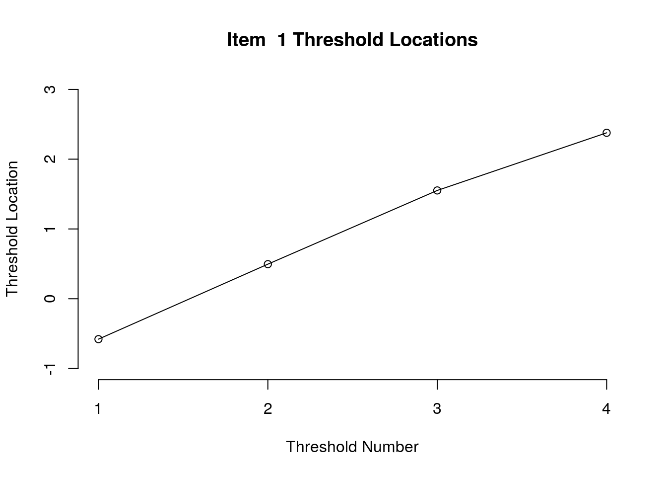
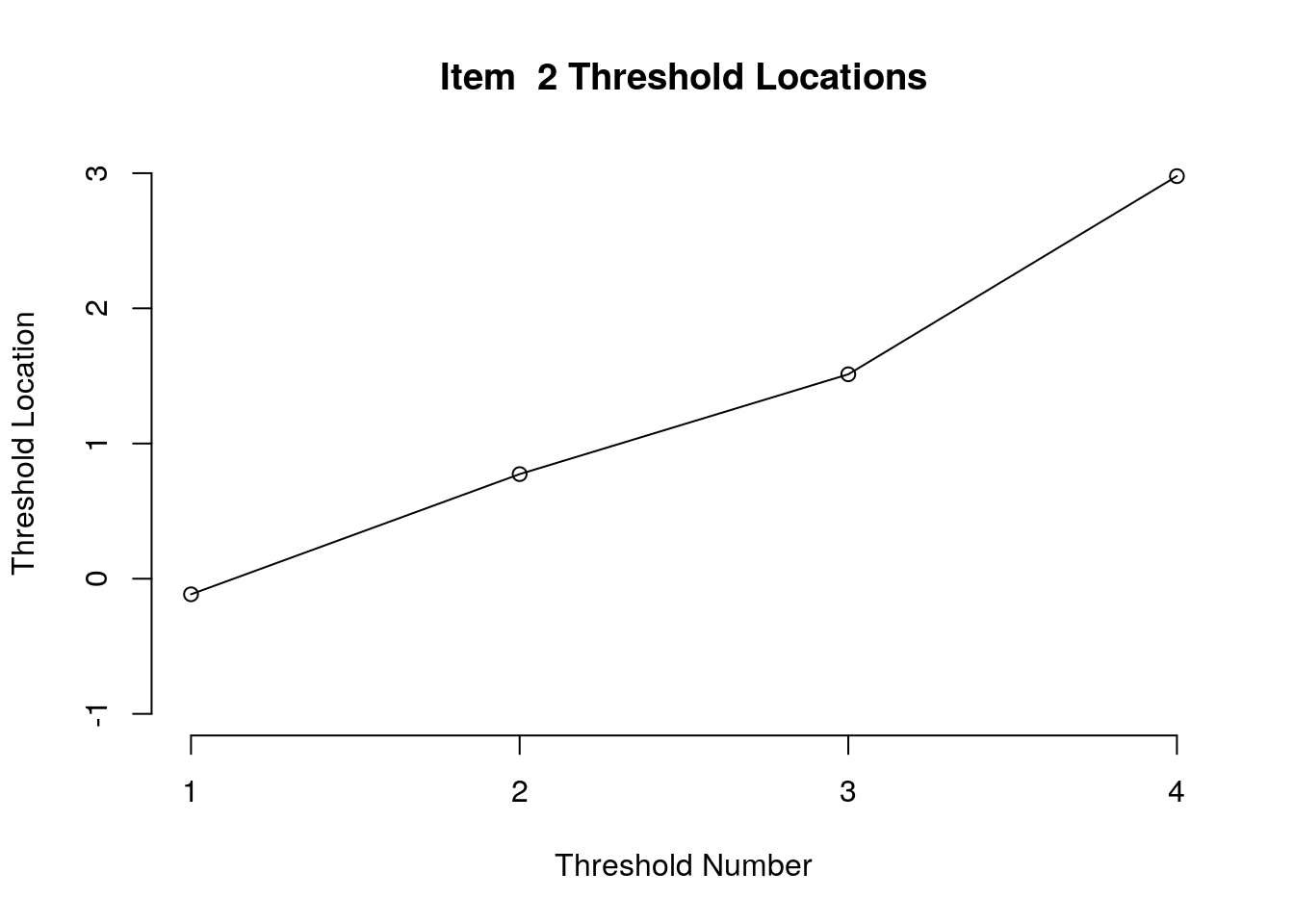
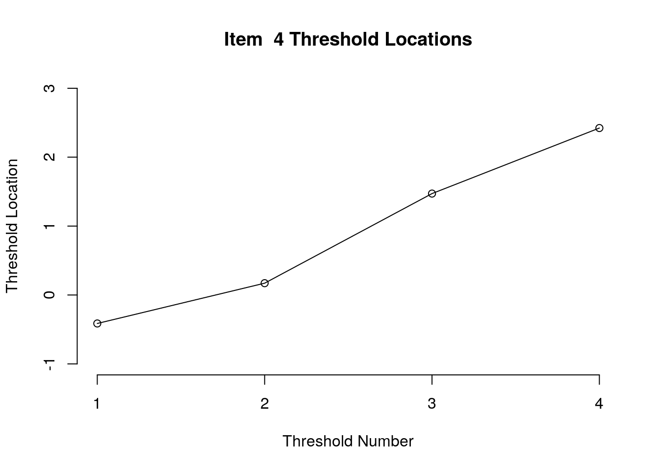
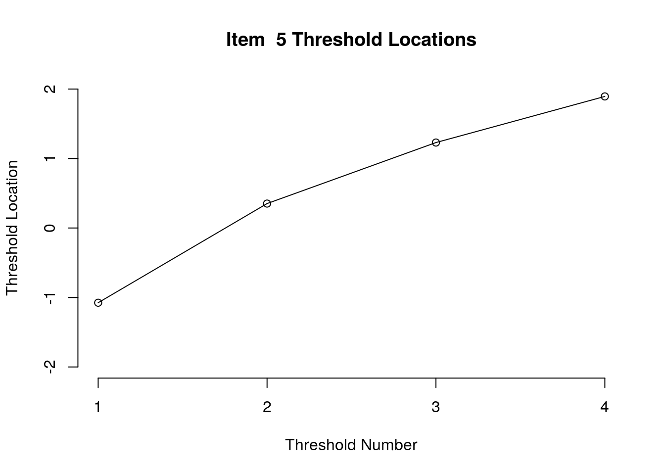

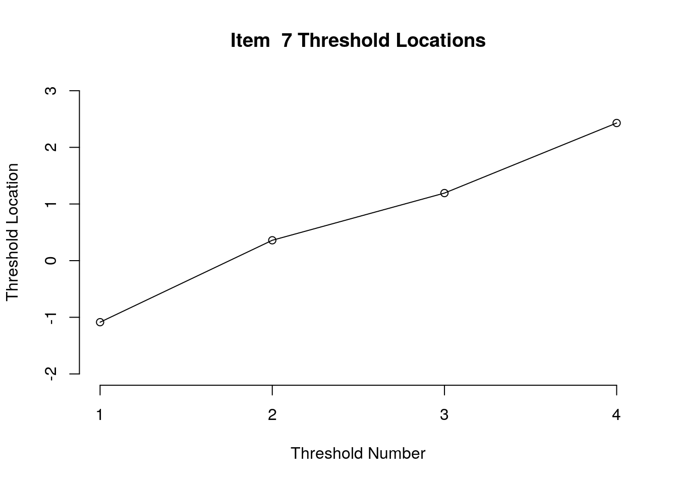

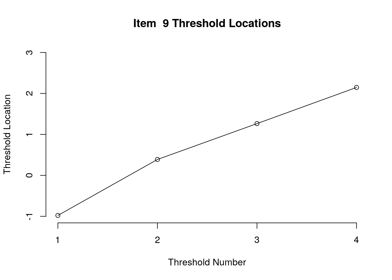
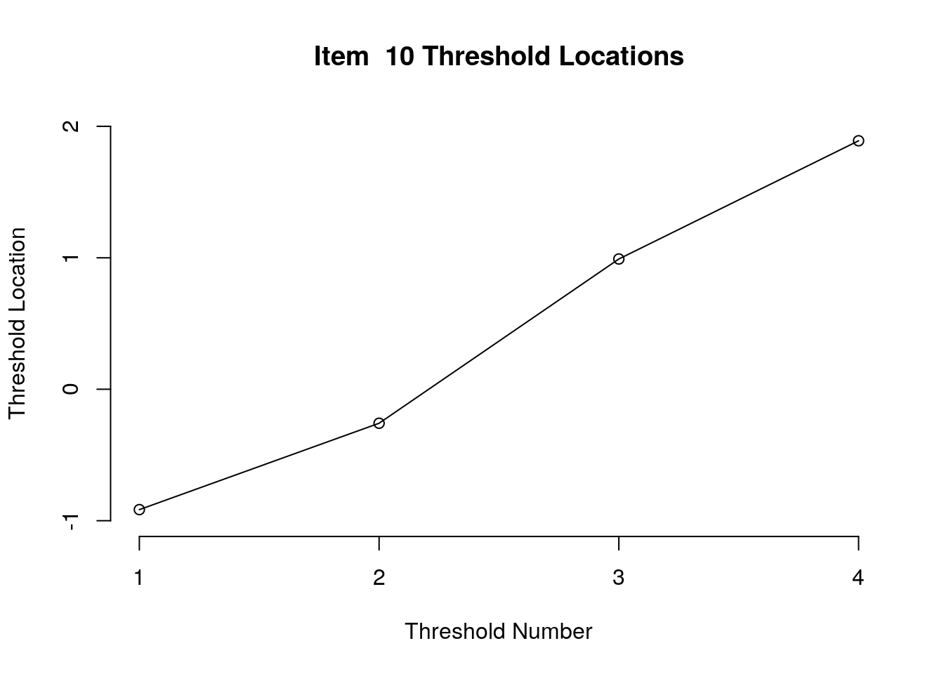
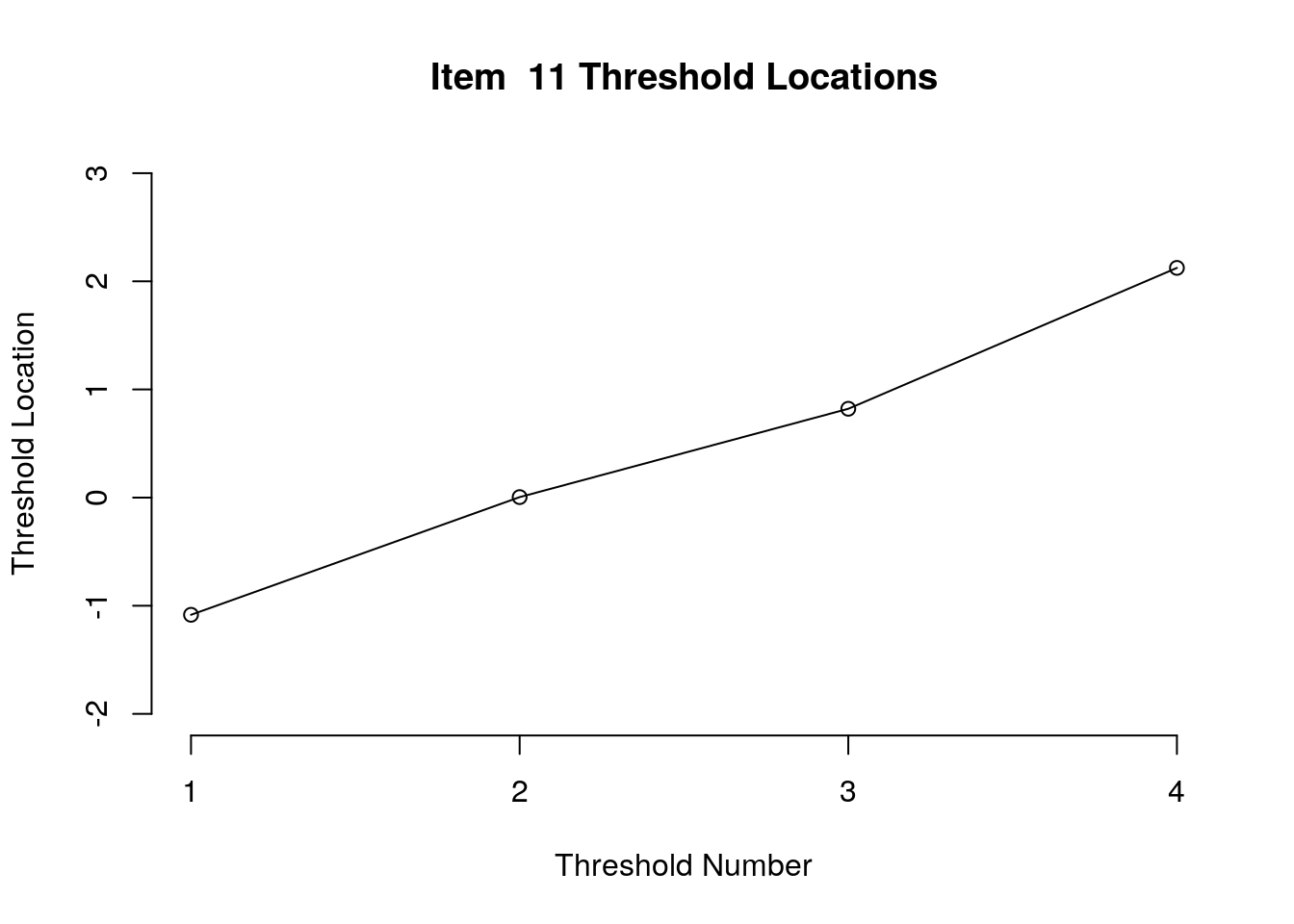

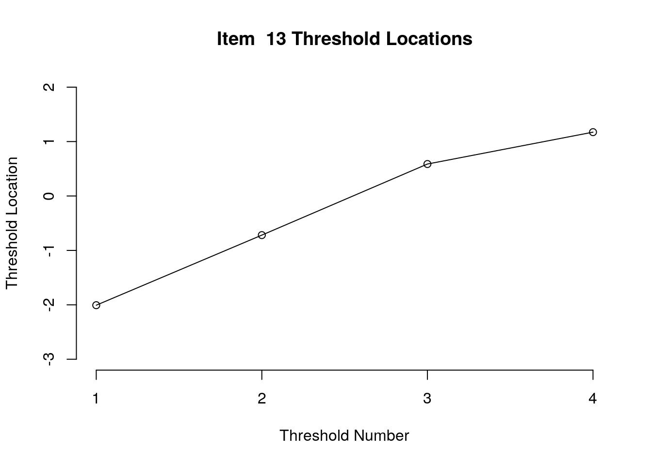

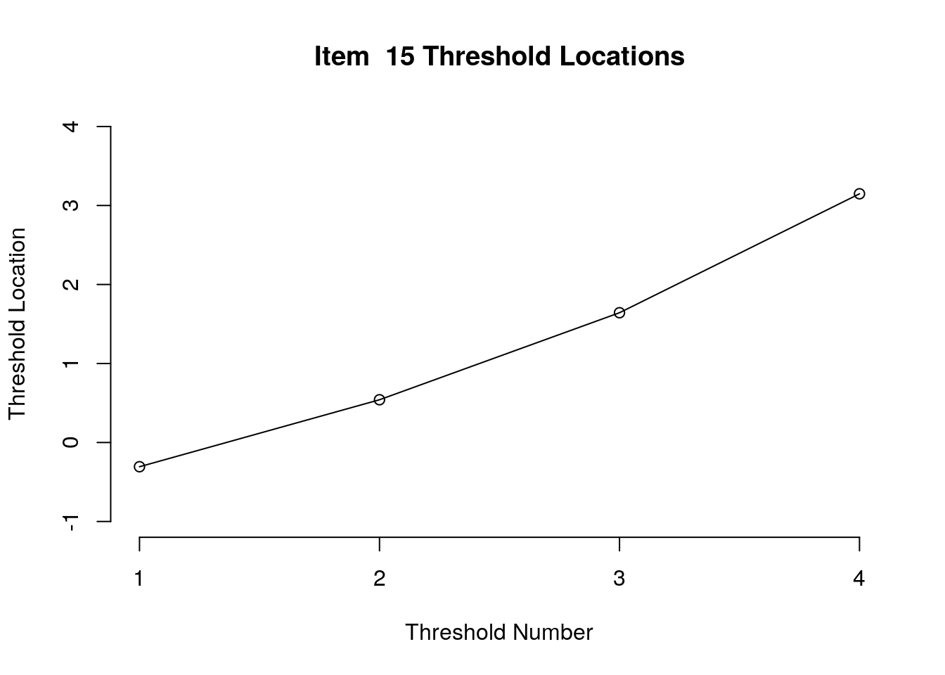
Running the above code will generate plots for each item that show the estimated location for each threshold.
Use the arrow buttons in the Plots window to navigate through the plots and examine the plots for evidence of non-decreasing threshold locations on the y-axis as the thresholds progress along the x-axis.
You can also check the distance between the threshold locations for evidence of distinct categories.
You can export the item and threshold location estimates for use in reporting
9.2.4 Examine Category Probability curves
Examine category probability curves for evidence of distinct and ordered categories.
# The function below that finds the threshold values specific to each item and plots them.
responses <- survey.responses # update to data object if using with other dataset!
model.results <- PC_model # update to model object if using with other dataset!
for(item.number in 1:ncol(survey.responses)){
  plotICC(model.results, item.subset = item.number)
}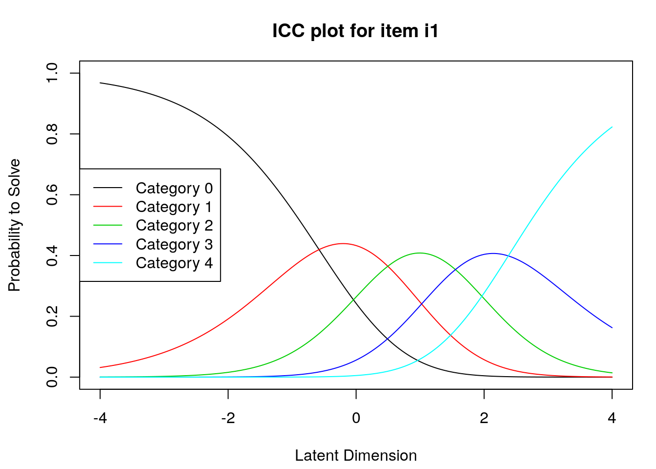
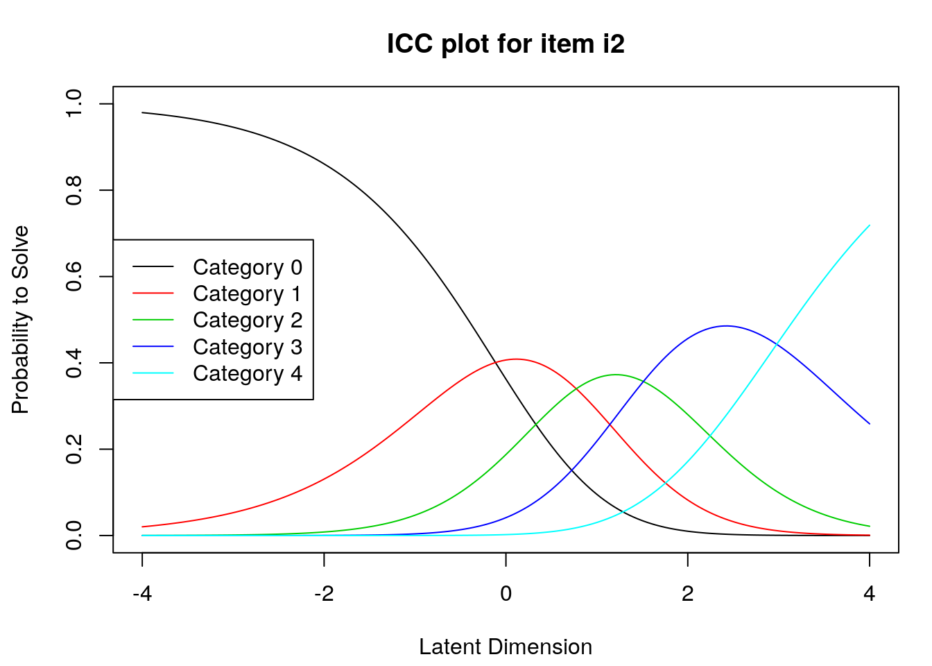
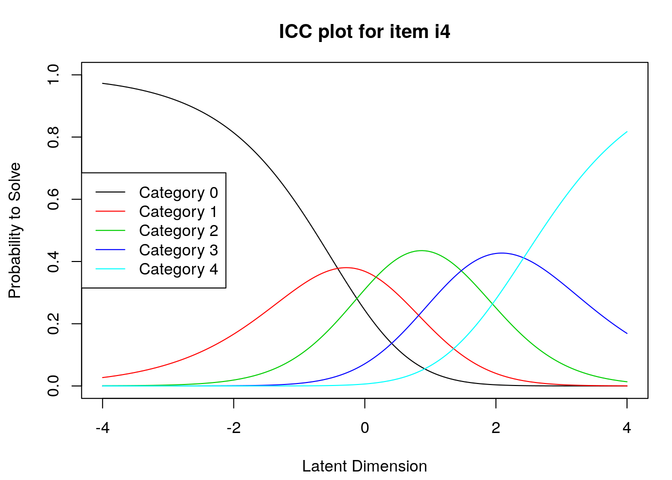

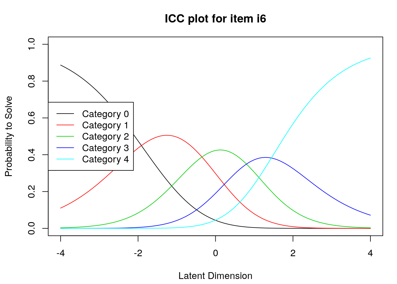
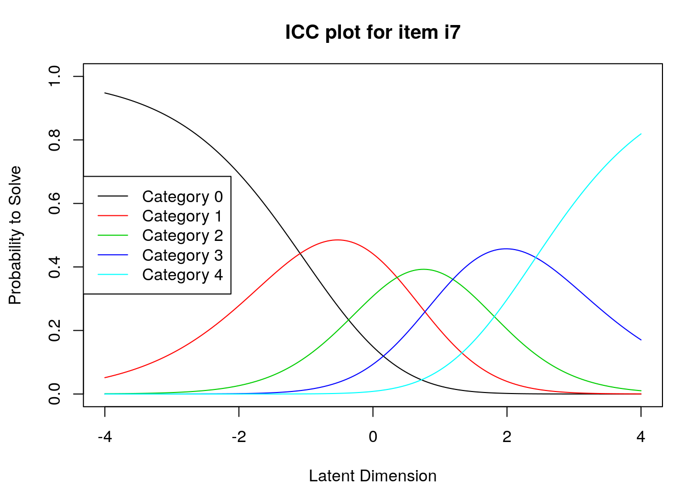

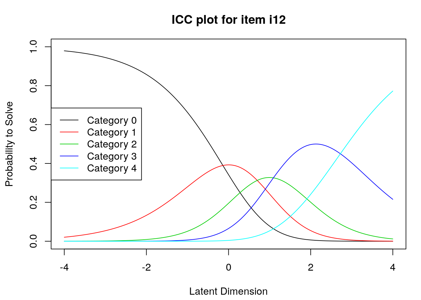
The code above will produce category probability plots in the Plots window.
- Use the arrow buttons in the Plots window to navigate through the plots and examine the plots for evidence of:
- Ordered category curves
- Distinct (modal) categories
9.3 Example APA-format Results section for rating scale analysis
We analyzed 350 participants’ responses to a 15-item survey that included items with five ordered categories (\(X\) = 0, 1, 2, 3, or 4) for evidence of useful rating scale category functioning. Specifically, following Linacre (2002) and Engelhard and Wind (2018), we examined the survey item responses for evidence of directional orientation with the latent variable and distinct categories on the construct. So that we could consider category functioning specific to each item with the most diagnostic utility, we used the Partial Credit Model (Masters, 1982) to analyze the data. We conducted the analyses using the Extended Rasch Models (“eRm”) package (Mair, Hatzinger, & Maier, 2020) for R.
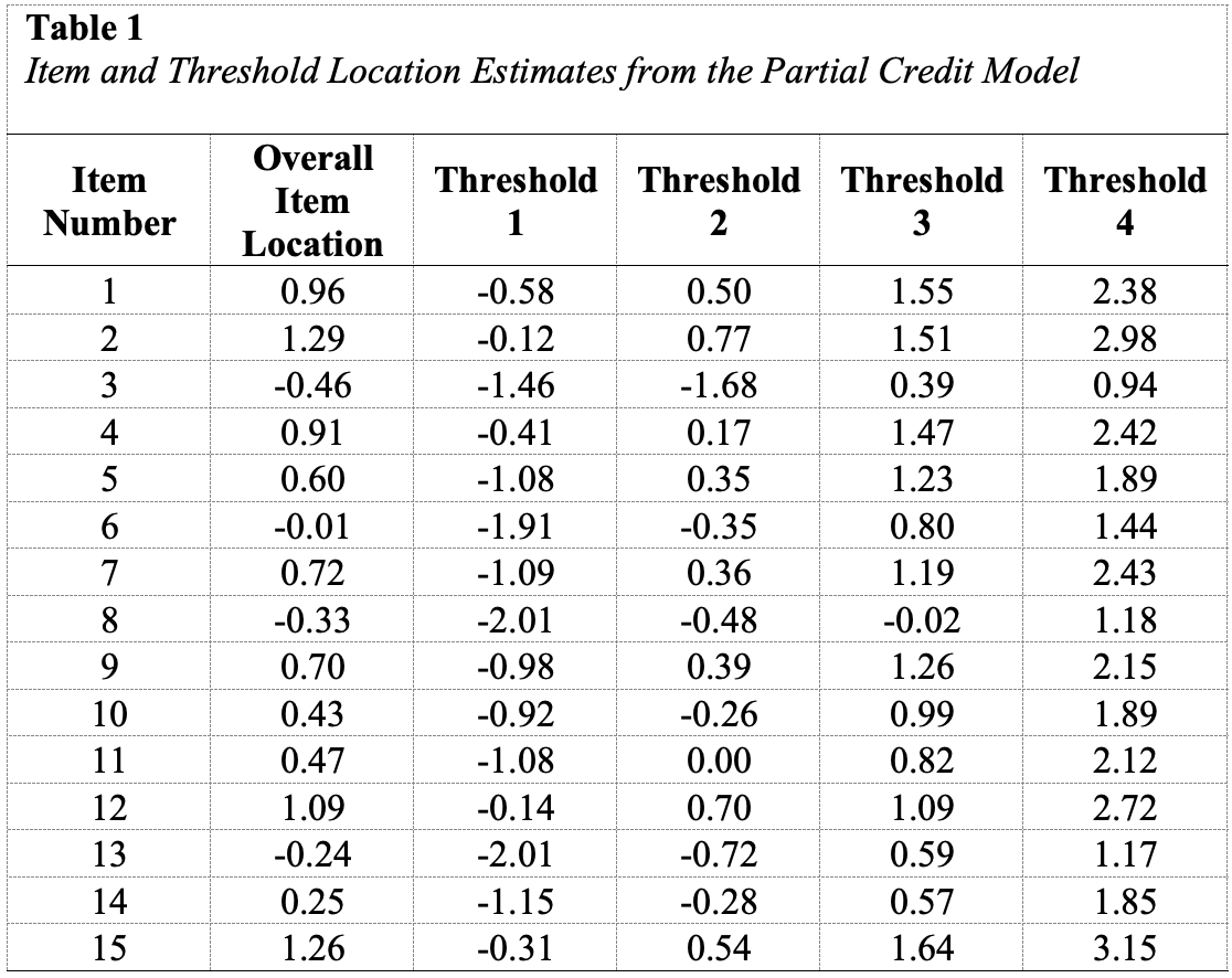
Table1:Item and Threshold Location Estimates from the Partial Credit Model
Participant responses to all 15 items included observations in all five rating scale categories. All of the items included at least 10 responses in each category except for the lowest rating scale category (\(X\) = 0) for Item 3 (frequency = 8), Item 8 (frequency = 9), and Item 13 (frequency = 9). In a future administration of this survey, researchers may consider reducing the scale length for these items to avoid unstable estimates.
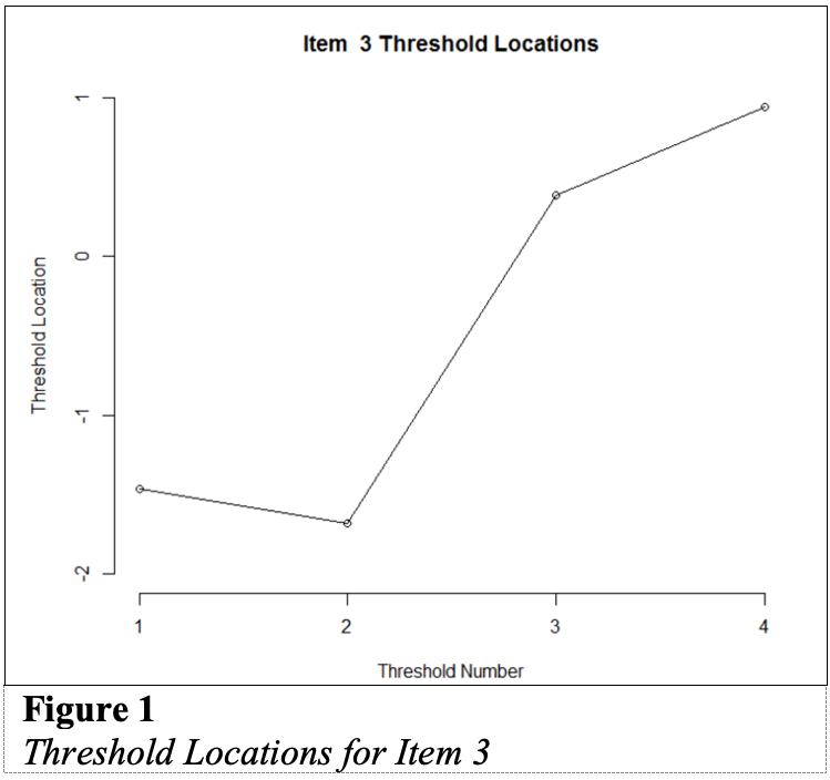
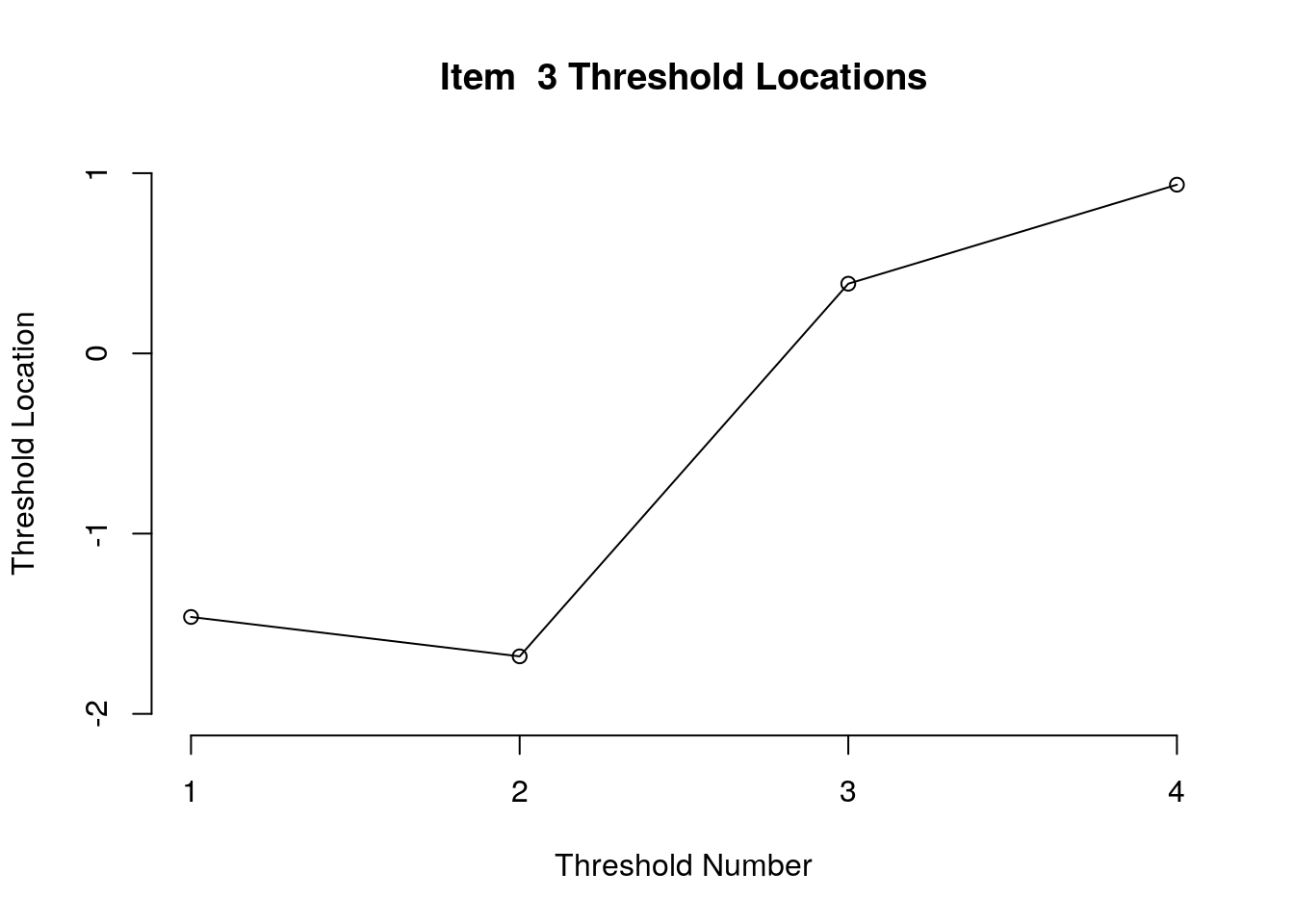
Figure 1:Threshold Locations for Item3
First, we examined the estimated threshold locations for each item for evidence of directional orientation with the latent variable (i.e., non-decreasing locations as categories increase). Because all of the items included responses in five categories, there were four threshold estimates for each item (τi1, τi2, τi3, τi4). Accordingly, we examined whether τi1 ≤ τi2, τi2 ≤ τi3, and τi3 ≤ τi4 for each item. Table 1 includes the threshold estimates for each item, along with the overall item location estimate. For Item 3, the first and second threshold were disordered (τ3,1 = -1.46, τ3,2 = -1.68; see Figure 1). For all of the other items, the thresholds were ordered as expected given the ordinal rating scale categories.
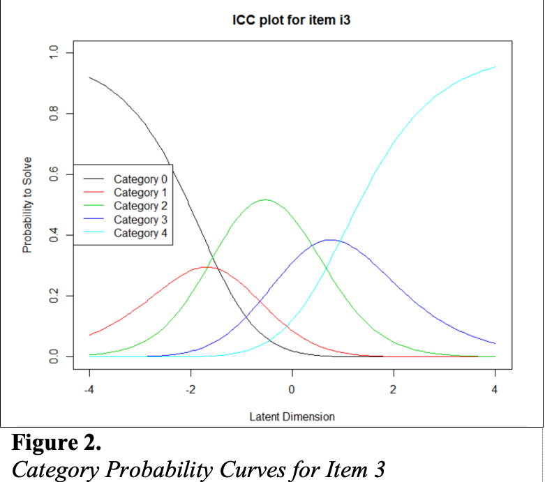
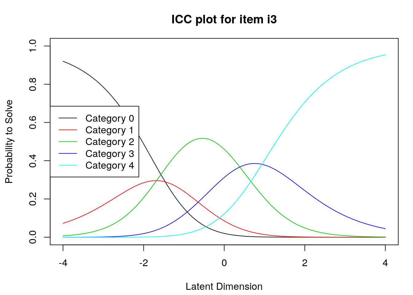
Figure 2: Category Probability Curves for Item 3
Next, we examined category probability curves for evidence that the rating scale categories were ordered as expected (non-decreasing threshold locations over increasing categories) and distinct for each item. Distinct categories imply that each rating scale category describes a meaningful range of locations on the logit scale that represents the construct. The categories appeared to function as expected for all of the items except Item 3 (see Figure 2). For this item, the first and second rating scale categories were disordered.
9.4 References
Andrich, D. A. (1978). A rating formulation for ordered response categories. Psychometrika, 43(4), 561–573. https://doi.org/10.1007/BF02293814
Engelhard, G., & Wind, S. A. (2018). Invariant measurement with raters and rating scales: Rasch models for rater-mediated assessments. Taylor & Francis.
Linacre, J. M. (2002). Optimizing rating scale category effectiveness. Journal of Applied Measurement, 3(1), 85–106.
Masters, G. N. (1982). A Rasch model for partial credit scoring. Psychometrika, 47(2), 149–174. https://doi.org/10.1007/BF02296272
Mair, P., Hatzinger, R., & Maier M. J. (2020). eRm: Extended Rasch Modeling. 1.0-1. https://cran.r-project.org/package=eRm