Chapter 6 Partial Credit Model
6.1 Partial Credit Model
6.1.1 Recall: Rating Scale Model Key Features
Same rating scale category structure across items
Same Distance between categories on the logit scale
Same number of categories across items
Thresholds can be disordered
6.1.2 Motivation for the Partial Credit (PC) Model
Some measurement contexts require multiple scale lengths
Sometimes categories are not observed for certain items (or used by individual raters)
Facilitates the empirical investigation of a common rating scale structure across items
6.1.3 Partial Credit Model Formula
The Partial Credit Model Masters, 1982 is generalization of the dichotomous Rasch Model. It provides estimates of Person locations, Item difficulties, and Thresholds specific to each item.
Partial Credit Model Equation
\[ln\left[\frac{P_{n_i(xi=k)}}{P_{n_i(xi=k-1)}}\right]=\theta_{n}-\delta_{i}-\tau_{ik}\]
In the PC model, Thresholds(\(τ_{k}\)) are estimated empirically for each element of one facet, such as items. They are not necessarily evenly spaced or ordered as expected. In contrast to the RS model, the location and relative distance between thresholds is estimated separately for each item.
6.2 R-Lab: Rasch Partial Credit Model with “eRm” package
For the Partial Credit Model, we will continue to work with the subset of the Braun (1988) essay data that we explored in the last Chapter. In this case, we will use “eRm” package.
6.2.1 Prepare the R package & the data
library(readr) # To import the data
library(eRm) # For running the Partial Credit Model
library(plyr) # For plot the Item characteristic curves
library(WrightMap)# For plot the variable map
Data Information
The original data collection design is described by Braun (1988). The original dataset includes ratings for 32 students by 12 raters on three separate essay compositions. For this lab, we will look at the data from Essay 1. For ease of interpretation, the essay ratings from the original dataset have been recoded from nine categories to three categories (0 = low achievement, 1 = middle achievement; 2 = high achievement).
In our analysis, we will treat the 12 raters as 12 polytomous “items” that share the three-category rating scale structure.
Raters with high “difficulty” calibrations can be interpreted as severe – these raters assign low scores more often. Raters with low “difficulty” calibrations can be interpreted as lenient – these raters assign high scores more often.
## # A tibble: 6 x 13
##   Student rater_1 rater_2 rater_3 rater_4 rater_5 rater_6 rater_7 rater_8
##     <dbl>   <dbl>   <dbl>   <dbl>   <dbl>   <dbl>   <dbl>   <dbl>   <dbl>
## 1       1       2       2       1       2       3       2       3       3
## 2       2       2       2       2       2       2       1       2       2
## 3       3       2       1       2       2       2       2       1       2
## 4       4       1       2       2       2       1       2       1       1
## 5       5       2       2       1       2       2       3       2       2
## 6       6       2       2       2       3       2       2       3       2
## # … with 4 more variables: rater_9 <dbl>, rater_10 <dbl>, rater_11 <dbl>,
## # rater_12 <dbl>## Student rater_1 rater_2 rater_3 rater_4
## Min. : 1.00 Min. :1.000 Min. :1.00 Min. :1.000 Min. :1.00
## 1st Qu.: 8.75 1st Qu.:1.750 1st Qu.:1.75 1st Qu.:1.000 1st Qu.:2.00
## Median :16.50 Median :2.000 Median :2.00 Median :2.000 Median :2.00
## Mean :16.50 Mean :1.781 Mean :1.75 Mean :1.688 Mean :2.25
## 3rd Qu.:24.25 3rd Qu.:2.000 3rd Qu.:2.00 3rd Qu.:2.000 3rd Qu.:3.00
## Max. :32.00 Max. :3.000 Max. :2.00 Max. :3.000 Max. :3.00
## rater_5 rater_6 rater_7 rater_8
## Min. :1.000 Min. :1.000 Min. :1.000 Min. :1.000
## 1st Qu.:2.000 1st Qu.:1.750 1st Qu.:1.000 1st Qu.:1.000
## Median :2.000 Median :2.000 Median :2.000 Median :2.000
## Mean :1.875 Mean :1.812 Mean :1.969 Mean :1.688
## 3rd Qu.:2.000 3rd Qu.:2.000 3rd Qu.:3.000 3rd Qu.:2.000
## Max. :3.000 Max. :3.000 Max. :3.000 Max. :3.000
## rater_9 rater_10 rater_11 rater_12
## Min. :1.000 Min. :1.000 Min. :1.000 Min. :1.000
## 1st Qu.:1.000 1st Qu.:2.000 1st Qu.:2.000 1st Qu.:2.000
## Median :2.000 Median :2.000 Median :2.000 Median :2.000
## Mean :1.875 Mean :2.031 Mean :1.938 Mean :2.094
## 3rd Qu.:2.000 3rd Qu.:2.000 3rd Qu.:2.000 3rd Qu.:2.000
## Max. :3.000 Max. :3.000 Max. :3.000 Max. :3.0006.2.2 R-Lab: Partial Credit Model with “eRm” package
# Run the Partial Credit Model
PC_model <- PCM(PC_data_balanced)
# Check the result
summary(PC_model)
##
## Results of PCM estimation:
##
## Call: PCM(X = PC_data_balanced)
##
## Conditional log-likelihood: -176.2042
## Number of iterations: 85
## Number of parameters: 22
##
## Item (Category) Difficulty Parameters (eta): with 0.95 CI:
## Estimate Std. Error lower CI upper CI
## rater_1.c2 3.431 1.089 1.296 5.565
## rater_2.c1 -1.037 0.479 -1.976 -0.099
## rater_3.c1 -0.193 0.436 -1.048 0.662
## rater_3.c2 3.394 0.854 1.720 5.069
## rater_4.c1 -3.621 1.007 -5.594 -1.647
## rater_4.c2 -1.933 1.032 -3.957 0.090
## rater_5.c1 -1.481 0.508 -2.476 -0.485
## rater_5.c2 2.235 0.878 0.513 3.957
## rater_6.c1 -1.002 0.471 -1.925 -0.079
## rater_6.c2 2.679 0.863 0.987 4.371
## rater_7.c1 -0.332 0.483 -1.279 0.616
## rater_7.c2 1.077 0.620 -0.138 2.292
## rater_8.c1 -0.193 0.436 -1.048 0.662
## rater_8.c2 3.394 0.854 1.720 5.069
## rater_9.c1 -0.463 0.465 -1.375 0.448
## rater_9.c2 1.689 0.660 0.395 2.984
## rater_10.c1 -2.422 0.641 -3.679 -1.165
## rater_10.c2 0.484 0.822 -1.126 2.095
## rater_11.c1 -1.741 0.538 -2.796 -0.686
## rater_11.c2 1.505 0.805 -0.073 3.084
## rater_12.c1 -3.691 1.001 -5.653 -1.730
## rater_12.c2 -0.761 1.088 -2.894 1.372
##
## Item Easiness Parameters (beta) with 0.95 CI:
## Estimate Std. Error lower CI upper CI
## beta rater_1.c1 1.020 0.469 0.102 1.939
## beta rater_1.c2 -3.431 1.089 -5.565 -1.296
## beta rater_2.c1 1.037 0.479 0.099 1.976
## beta rater_3.c1 0.193 0.436 -0.662 1.048
## beta rater_3.c2 -3.394 0.854 -5.069 -1.720
## beta rater_4.c1 3.621 1.007 1.647 5.594
## beta rater_4.c2 1.933 1.032 -0.090 3.957
## beta rater_5.c1 1.481 0.508 0.485 2.476
## beta rater_5.c2 -2.235 0.878 -3.957 -0.513
## beta rater_6.c1 1.002 0.471 0.079 1.925
## beta rater_6.c2 -2.679 0.863 -4.371 -0.987
## beta rater_7.c1 0.332 0.483 -0.616 1.279
## beta rater_7.c2 -1.077 0.620 -2.292 0.138
## beta rater_8.c1 0.193 0.436 -0.662 1.048
## beta rater_8.c2 -3.394 0.854 -5.069 -1.720
## beta rater_9.c1 0.463 0.465 -0.448 1.375
## beta rater_9.c2 -1.689 0.660 -2.984 -0.395
## beta rater_10.c1 2.422 0.641 1.165 3.679
## beta rater_10.c2 -0.484 0.822 -2.095 1.126
## beta rater_11.c1 1.741 0.538 0.686 2.796
## beta rater_11.c2 -1.505 0.805 -3.084 0.073
## beta rater_12.c1 3.691 1.001 1.730 5.653
## beta rater_12.c2 0.761 1.088 -1.372 2.8946.2.3 Wright Map & Expected Response Curves & Item characteristic curves
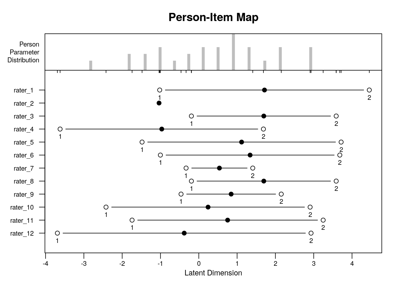
Wright Map or Variable Map
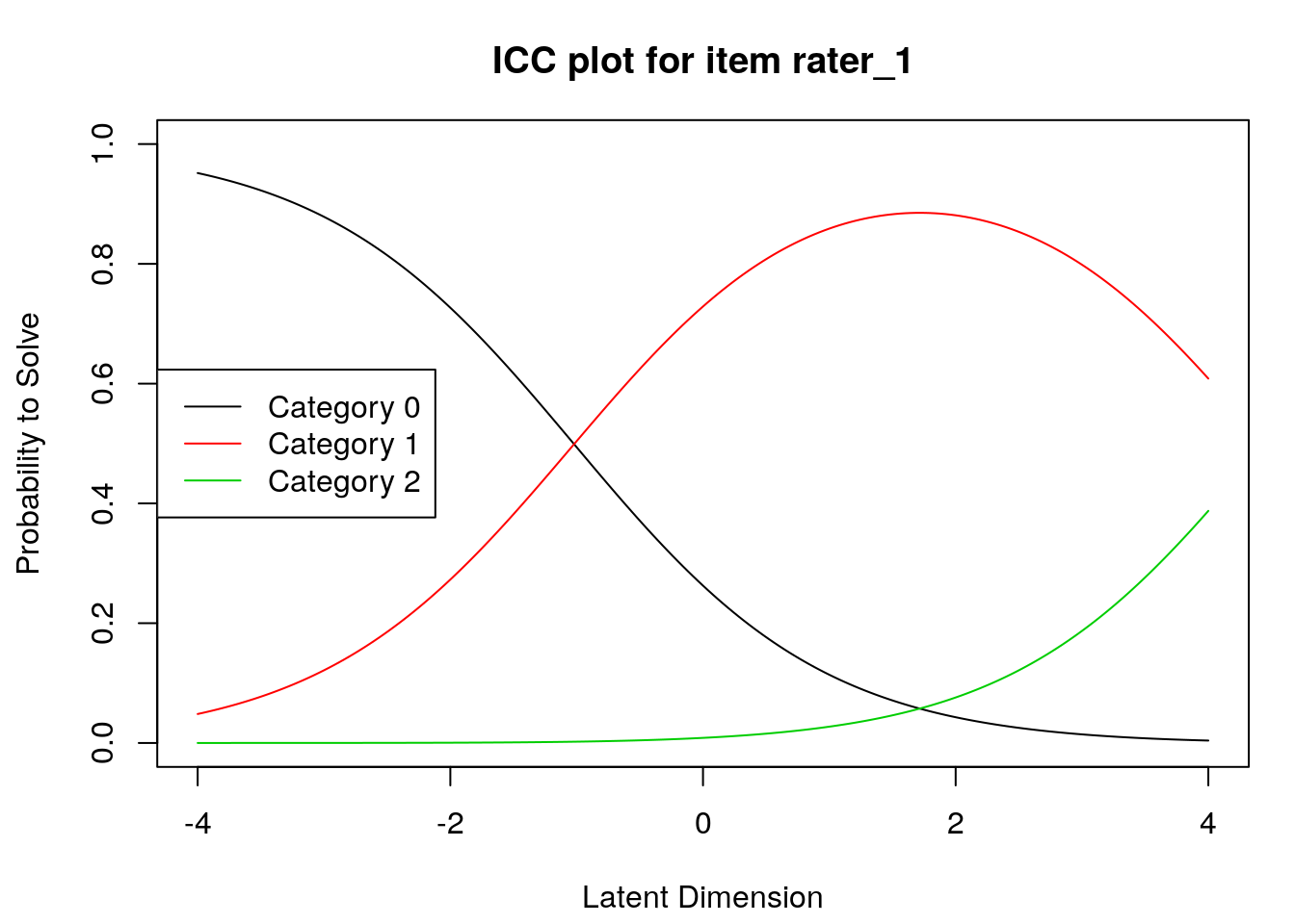
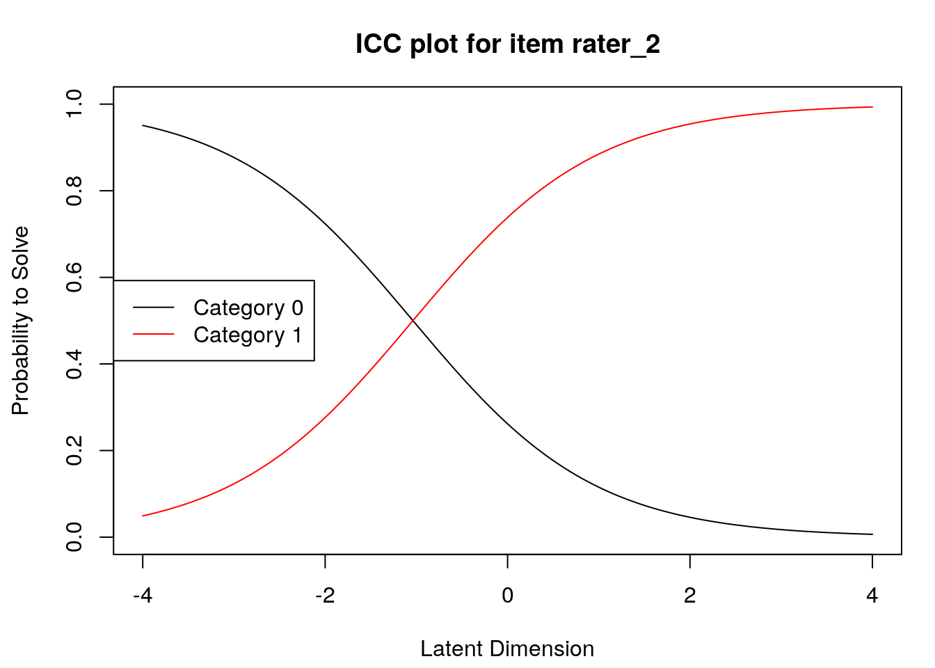
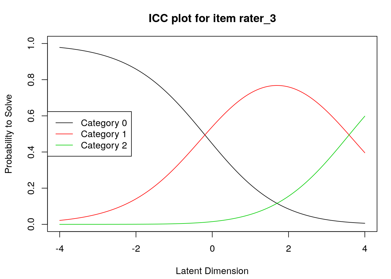
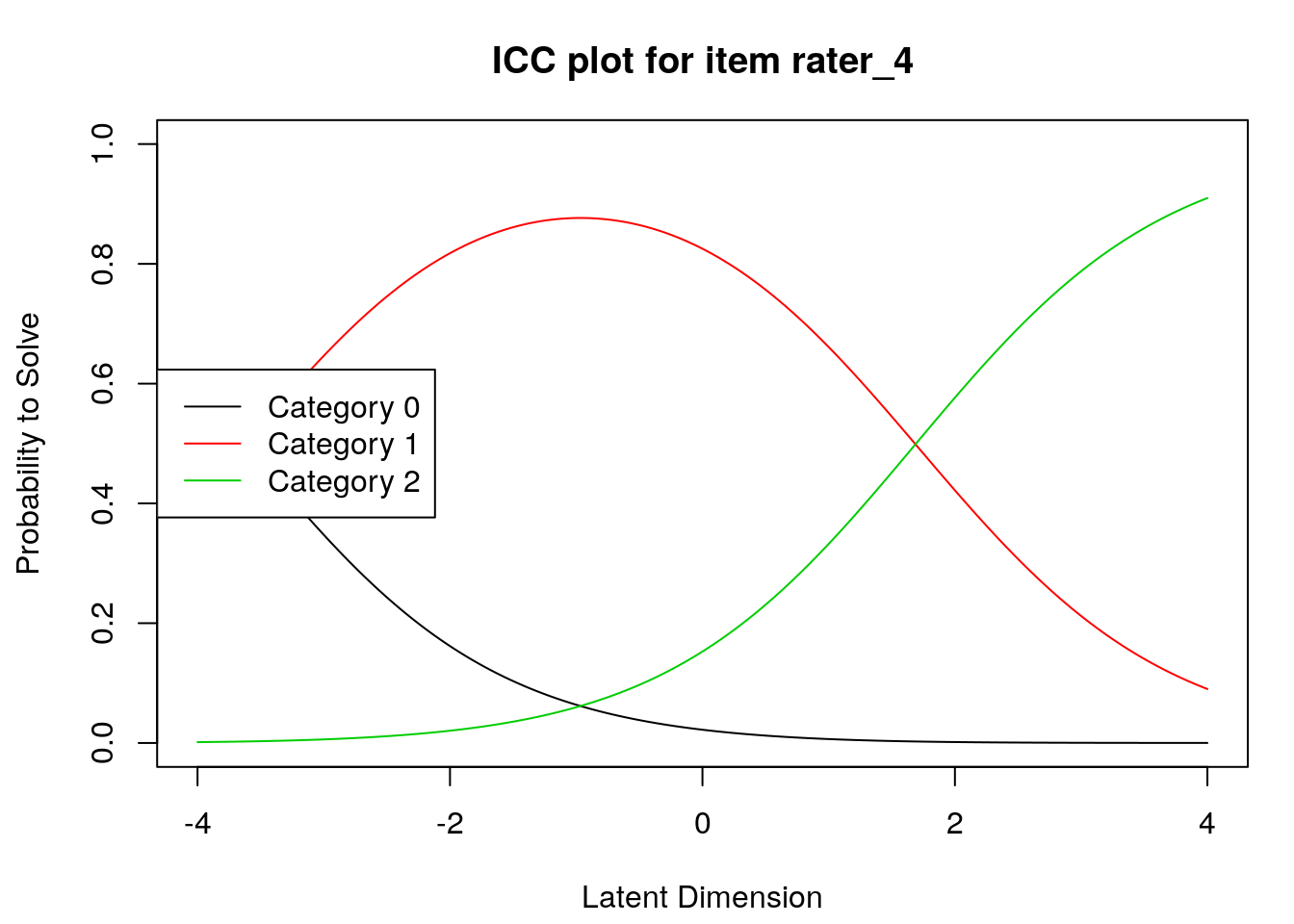
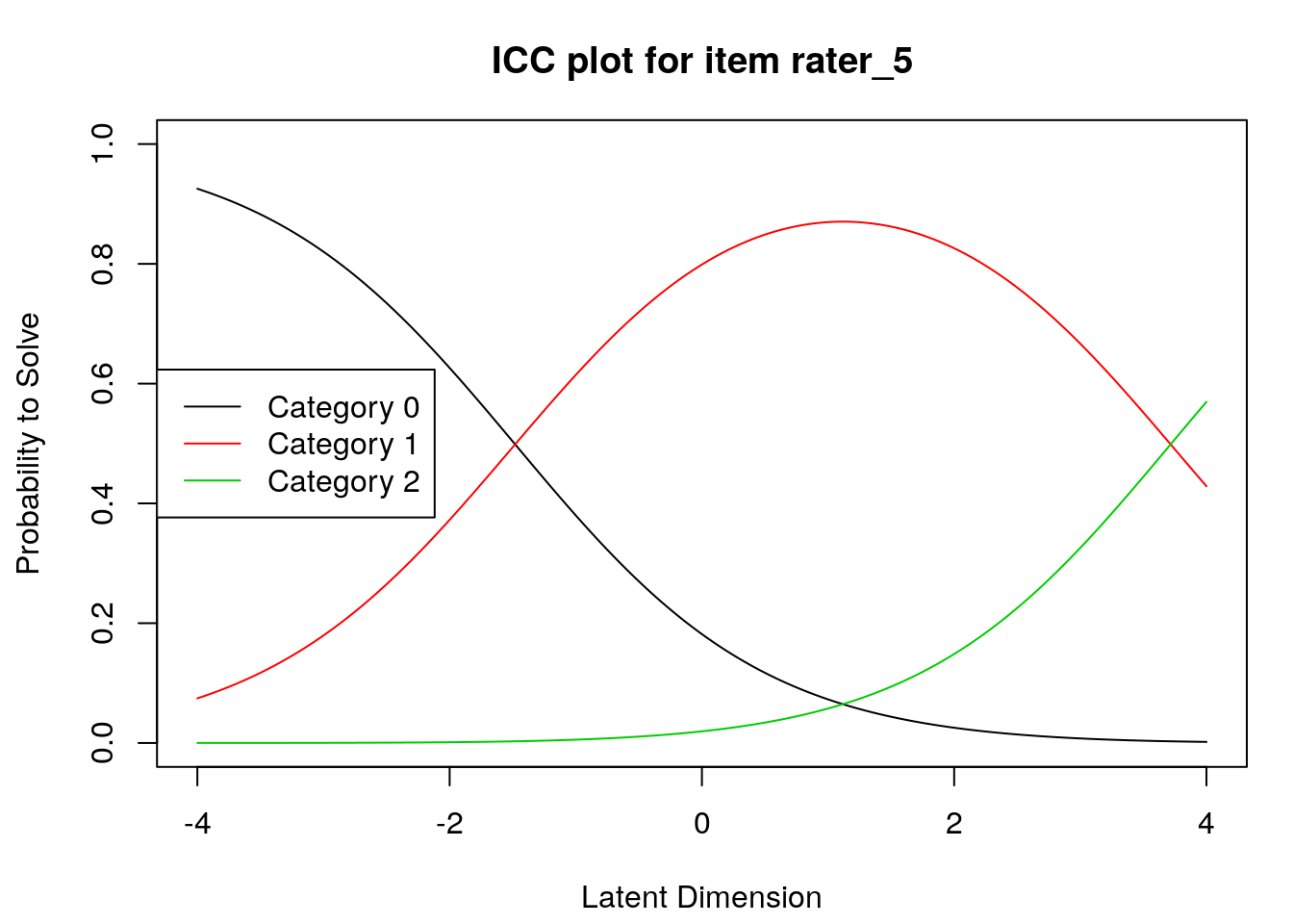
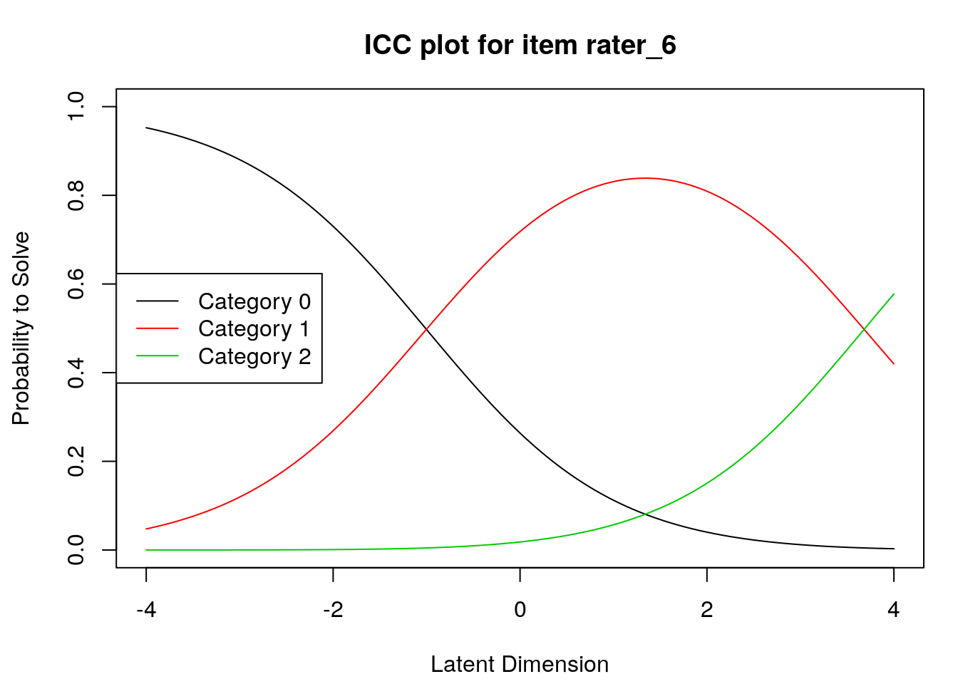
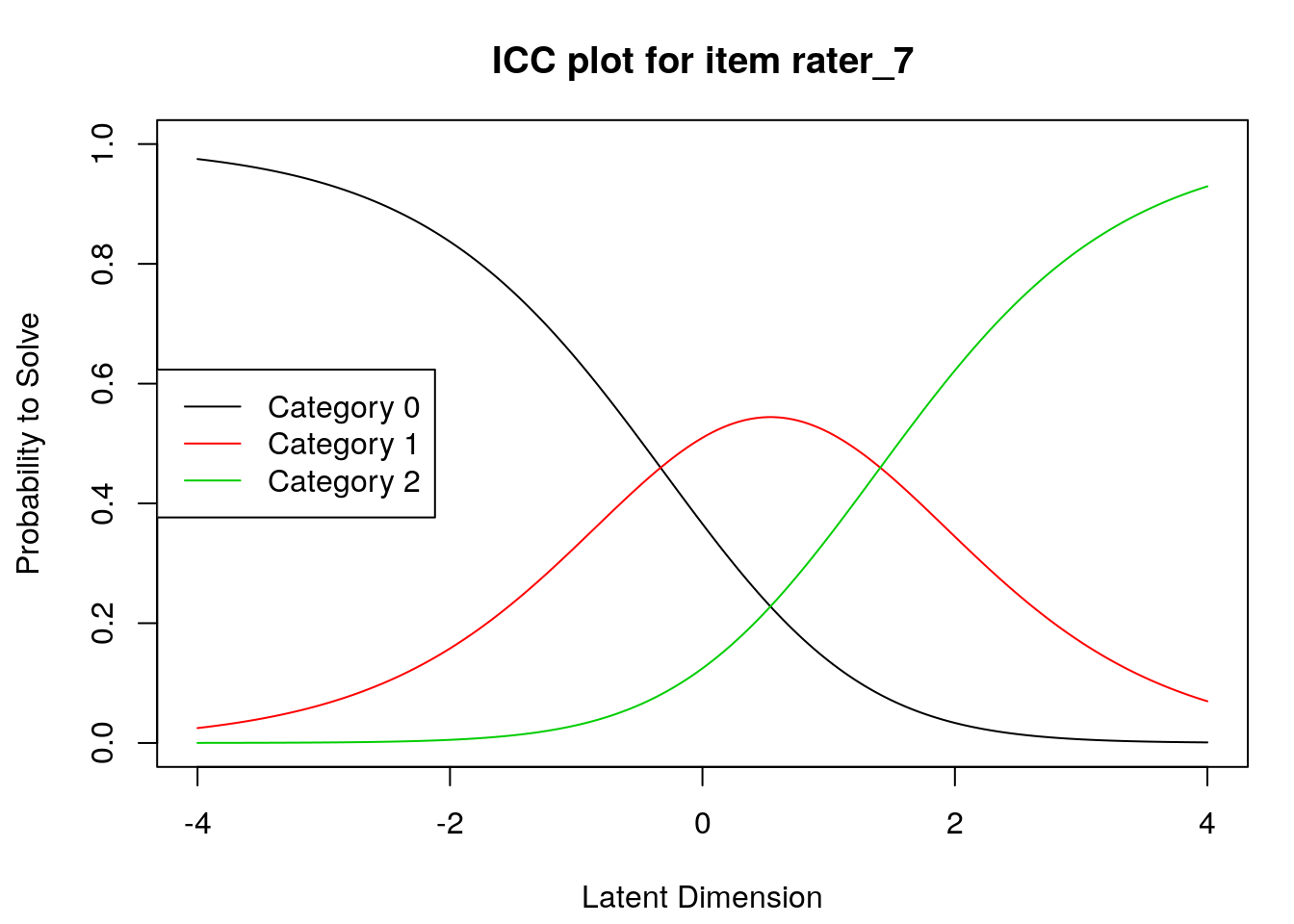
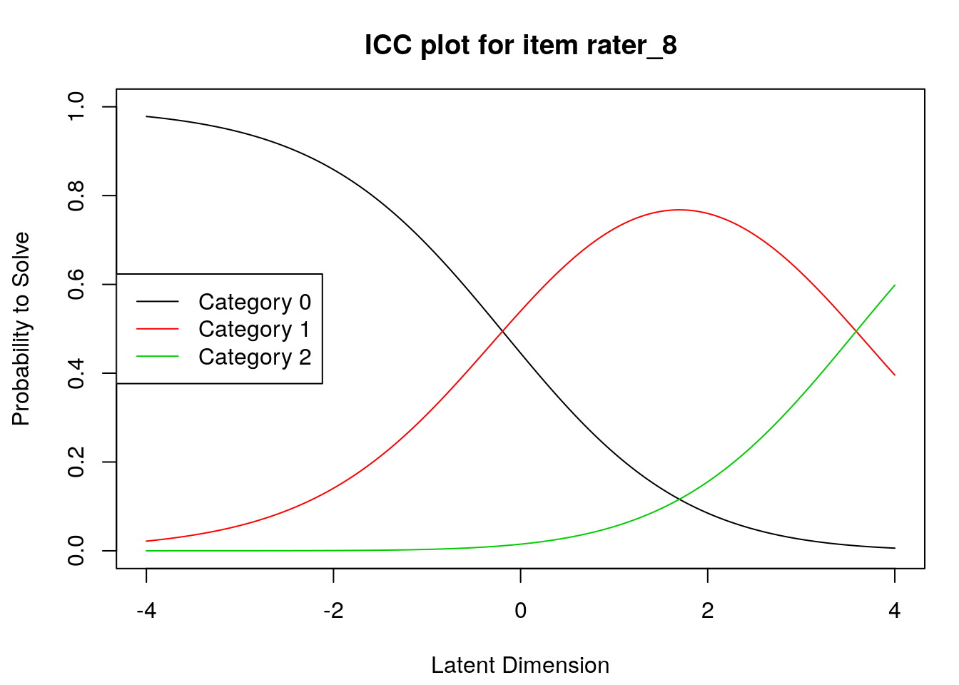
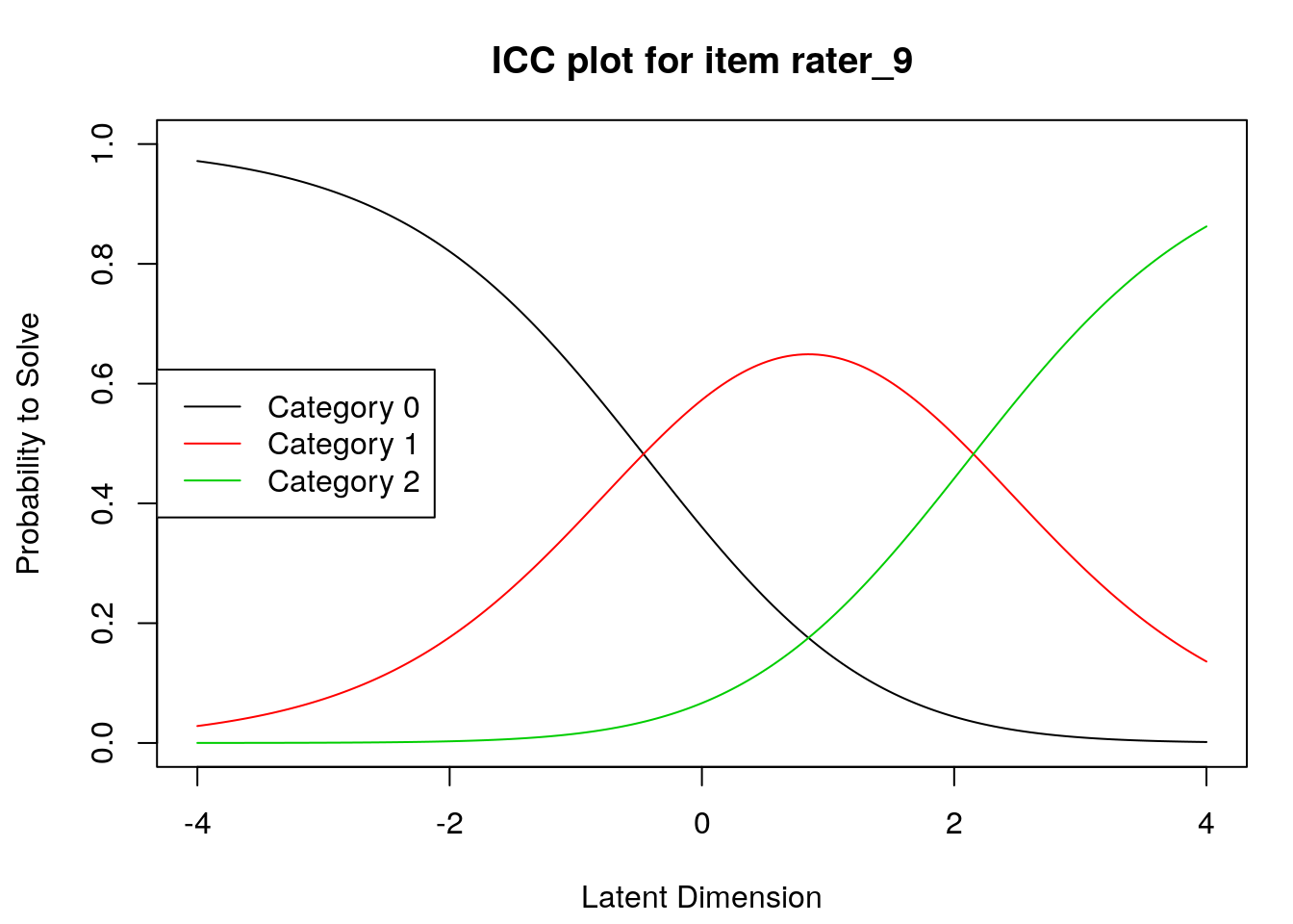
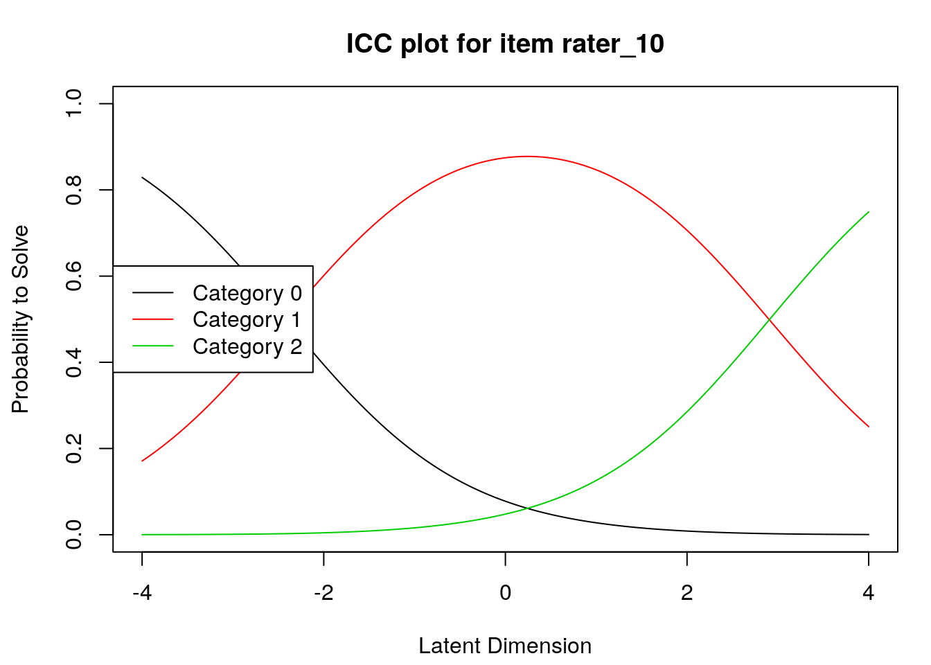
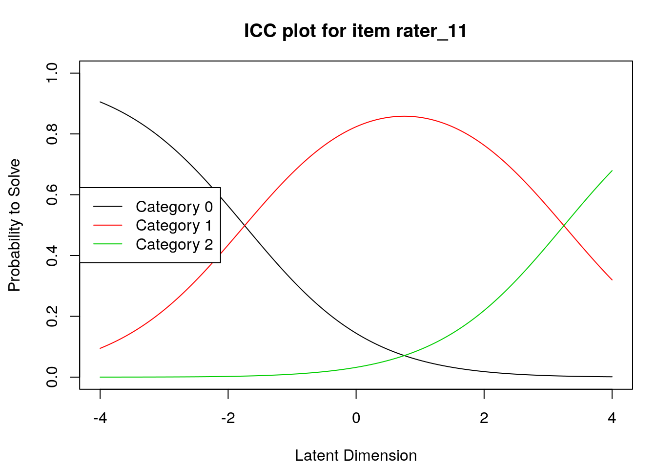
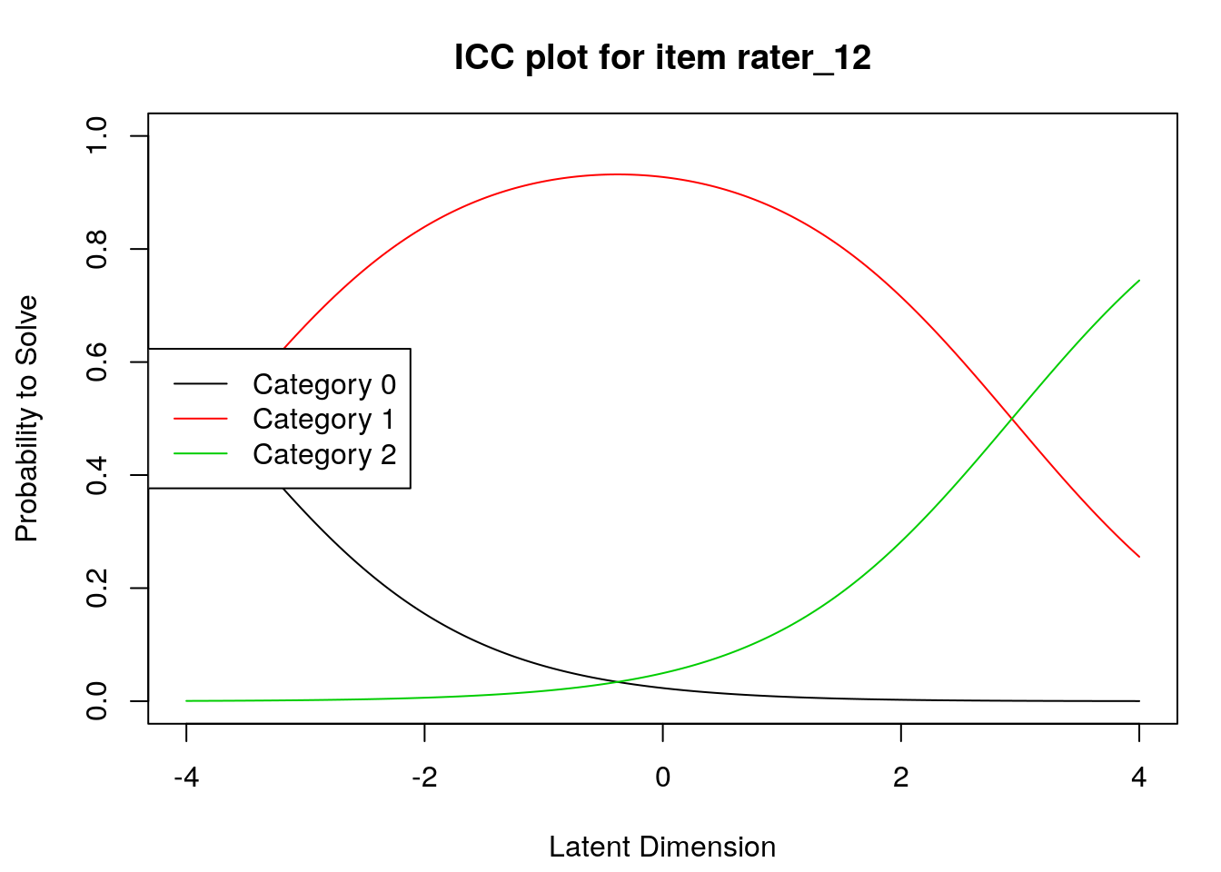
Item characteristic curves
6.2.4 Examine item difficulty and threshold SEs
##
## Design Matrix Block 1:
##          Location Threshold 1 Threshold 2
## rater_1   1.71533    -1.02044     4.45110
## rater_2  -1.03738    -1.03738          NA
## rater_3   1.69705    -0.19282     3.58692
## rater_4  -0.96654    -3.62052     1.68743
## rater_5   1.11751    -1.48079     3.71582
## rater_6   1.33961    -1.00214     3.68137
## rater_7   0.53860    -0.33161     1.40880
## rater_8   1.69705    -0.19282     3.58692
## rater_9   0.84473    -0.46316     2.15262
## rater_10  0.24219    -2.42170     2.90607
## rater_11  0.75273    -1.74141     3.24687
## rater_12 -0.38032 -3.69109 2.93045## Location Threshold 1 Threshold 2
## rater_1 1.7153307 -1.0204400 4.451101
## rater_2 -1.0373790 -1.0373790 NA
## rater_3 1.6970522 -0.1928160 3.586920
## rater_4 -0.9665425 -3.6205191 1.687434
## rater_5 1.1175132 -1.4807928 3.715819
## rater_6 1.3396144 -1.0021416 3.681370
## rater_7 0.5385964 -0.3316063 1.408799
## rater_8 1.6970522 -0.1928160 3.586920
## rater_9 0.8447299 -0.4631578 2.152618
## rater_10 0.2421854 -2.4216996 2.906070
## rater_11 0.7527270 -1.7414141 3.246868
## rater_12 -0.3803220 -3.6910917 2.930448## thresh beta rater_1.c1 thresh beta rater_1.c2 thresh beta rater_2.c1
## 0.4685140 1.0382566 0.4788181
## thresh beta rater_3.c1 thresh beta rater_3.c2 thresh beta rater_4.c1
## 0.4362702 0.7916276 1.0069356
## thresh beta rater_4.c2 thresh beta rater_5.c1 thresh beta rater_5.c2
## 0.4715850 0.5078359 0.7766796
## thresh beta rater_6.c1 thresh beta rater_6.c2 thresh beta rater_7.c1
## 0.4710416 0.7807315 0.4833211
## thresh beta rater_7.c2 thresh beta rater_8.c1 thresh beta rater_8.c2
## 0.5116547 0.4362701 0.7916260
## thresh beta rater_9.c1 thresh beta rater_9.c2 thresh beta rater_10.c1
## 0.4651363 0.5557134 0.6412761
## thresh beta rater_10.c2 thresh beta rater_11.c1 thresh beta rater_11.c2
## 0.6006856 0.5382447 0.6666485
## thresh beta rater_12.c1 thresh beta rater_12.c2
## 1.0007812 0.59701506.2.5 Examine Person locations (theta) and SEs
# Standard errors for theta estimates:
person.locations.estimate <- person.parameter(PC_model)
summary(person.locations.estimate)
##
## Estimation of Ability Parameters
##
## Collapsed log-likelihood: -90.03962
## Number of iterations: 6
## Number of parameters: 13
##
## ML estimated ability parameters (without spline interpolated values):
## Estimate Std. Err. 2.5 % 97.5 %
## theta P1 2.9215618 0.6285533 1.68962010 4.1535036
## theta P2 0.1159553 0.6183290 -1.09594736 1.3278579
## theta P3 -0.2617525 0.6115686 -1.46040495 0.9368999
## theta P4 -1.0101623 0.6169495 -2.21936113 0.1990366
## theta P5 0.9042291 0.6366178 -0.34351886 2.1519770
## theta P6 1.3127857 0.6407989 0.05684305 2.5687285
## theta P7 1.3127857 0.6407989 0.05684305 2.5687285
## theta P8 0.9042291 0.6366178 -0.34351886 2.1519770
## theta P9 -0.6343992 0.6104489 -1.83085716 0.5620587
## theta P10 2.9215618 0.6285533 1.68962010 4.1535036
## theta P11 0.1159553 0.6183290 -1.09594736 1.3278579
## theta P12 0.5041406 0.6279373 -0.72659391 1.7348751
## theta P13 1.7229829 0.6392554 0.47006527 2.9759005
## theta P14 -1.3996406 0.6329278 -2.64015634 -0.1591248
## theta P15 2.1284749 0.6339777 0.88590145 3.3710484
## theta P16 0.9042291 0.6366178 -0.34351886 2.1519770
## theta P17 0.5041406 0.6279373 -0.72659391 1.7348751
## theta P18 -0.2617525 0.6115686 -1.46040495 0.9368999
## theta P19 2.9215618 0.6285533 1.68962010 4.1535036
## theta P20 0.5041406 0.6279373 -0.72659391 1.7348751
## theta P21 -1.0101623 0.6169495 -2.21936113 0.1990366
## theta P22 2.1284749 0.6339777 0.88590145 3.3710484
## theta P23 0.9042291 0.6366178 -0.34351886 2.1519770
## theta P24 -2.8215012 0.7705556 -4.33176236 -1.3112400
## theta P25 0.9042291 0.6366178 -0.34351886 2.1519770
## theta P26 2.1284749 0.6339777 0.88590145 3.3710484
## theta P27 -1.3996406 0.6329278 -2.64015634 -0.1591248
## theta P28 -1.8166969 0.6608117 -3.11186398 -0.5215298
## theta P29 -1.0101623 0.6169495 -2.21936113 0.1990366
## theta P30 0.1159553 0.6183290 -1.09594736 1.3278579
## theta P31 -1.8166969 0.6608117 -3.11186398 -0.5215298
## theta P32 1.3127857 0.6407989 0.05684305 2.5687285# Build a table for person locations
person_theta <- person.locations.estimate$theta.table
person_theta## Person Parameter NAgroup Interpolated
## P1 2.9215618 1 FALSE
## P2 0.1159553 1 FALSE
## P3 -0.2617525 1 FALSE
## P4 -1.0101623 1 FALSE
## P5 0.9042291 1 FALSE
## P6 1.3127857 1 FALSE
## P7 1.3127857 1 FALSE
## P8 0.9042291 1 FALSE
## P9 -0.6343992 1 FALSE
## P10 2.9215618 1 FALSE
## P11 0.1159553 1 FALSE
## P12 0.5041406 1 FALSE
## P13 1.7229829 1 FALSE
## P14 -1.3996406 1 FALSE
## P15 2.1284749 1 FALSE
## P16 0.9042291 1 FALSE
## P17 0.5041406 1 FALSE
## P18 -0.2617525 1 FALSE
## P19 2.9215618 1 FALSE
## P20 0.5041406 1 FALSE
## P21 -1.0101623 1 FALSE
## P22 2.1284749 1 FALSE
## P23 0.9042291 1 FALSE
## P24 -2.8215012 1 FALSE
## P25 0.9042291 1 FALSE
## P26 2.1284749 1 FALSE
## P27 -1.3996406 1 FALSE
## P28 -1.8166969 1 FALSE
## P29 -1.0101623 1 FALSE
## P30 0.1159553 1 FALSE
## P31 -1.8166969 1 FALSE
## P32 1.3127857 1 FALSE6.2.6 Exam the item and person fit statistics
##
## Itemfit Statistics:
##           Chisq df p-value Outfit MSQ Infit MSQ Outfit t Infit t Discrim
## rater_1  16.463 31   0.985      0.514     0.618   -1.726  -1.582   0.726
## rater_2  28.274 31   0.607      0.884     1.193   -0.042   0.822   0.366
## rater_3  39.505 31   0.141      1.235     1.229    0.920   0.974   0.357
## rater_4  25.803 31   0.731      0.806     0.821   -0.605  -0.702   0.582
## rater_5  27.703 31   0.636      0.866     0.878   -0.326  -0.379   0.549
## rater_6  38.967 31   0.154      1.218     1.176    0.810   0.738   0.333
## rater_7  14.923 31   0.993      0.466     0.508   -2.432  -2.570   0.845
## rater_8  23.143 31   0.844      0.723     0.799   -1.084  -0.826   0.671
## rater_9  49.382 31   0.019      1.543     1.324    2.009   1.358   0.336
## rater_10 18.362 31   0.965      0.574     0.725   -1.406  -0.997   0.635
## rater_11 28.200 31   0.611      0.881     0.827   -0.293  -0.605   0.546
## rater_12 29.993 31   0.518      0.937     0.987    0.006   0.069   0.353
item.fit.table <- cbind(item.fit[["i.outfitMSQ"]],item.fit[["i.infitMSQ"]],item.fit[["i.infitMSQ"]],item.fit[["i.infitZ"]])
pfit <- personfit(person.locations.estimate)
pfit##
## Personfit Statistics:
## Chisq df p-value Outfit MSQ Infit MSQ Outfit t Infit t
## P1 18.317 11 0.075 1.526 1.733 0.89 1.92
## P2 10.340 11 0.500 0.862 0.766 -0.10 -0.46
## P3 7.507 11 0.757 0.626 0.766 -0.70 -0.55
## P4 8.787 11 0.642 0.732 0.813 -0.52 -0.50
## P5 10.399 11 0.495 0.867 0.813 -0.05 -0.24
## P6 6.927 11 0.805 0.577 0.915 -0.67 -0.01
## P7 6.250 11 0.856 0.521 0.438 -0.82 -1.29
## P8 17.151 11 0.103 1.429 1.244 0.85 0.62
## P9 7.851 11 0.727 0.654 0.763 -0.68 -0.64
## P10 8.773 11 0.643 0.731 0.853 -0.21 -0.35
## P11 14.839 11 0.190 1.237 1.368 0.59 0.92
## P12 5.979 11 0.875 0.498 0.383 -0.94 -1.60
## P13 9.738 11 0.554 0.811 0.800 -0.16 -0.30
## P14 12.314 11 0.341 1.026 1.074 0.20 0.33
## P15 14.142 11 0.225 1.179 1.549 0.48 1.24
## P16 8.965 11 0.625 0.747 0.834 -0.30 -0.19
## P17 39.175 11 0.000 3.265 2.312 2.81 2.22
## P18 8.442 11 0.673 0.704 0.796 -0.49 -0.45
## P19 16.823 11 0.113 1.402 1.555 0.75 1.54
## P20 6.893 11 0.808 0.574 0.861 -0.73 -0.16
## P21 6.922 11 0.805 0.577 0.662 -0.99 -1.07
## P22 3.572 11 0.981 0.298 0.366 -1.52 -1.83
## P23 5.636 11 0.896 0.470 0.792 -0.98 -0.29
## P24 15.824 11 0.148 1.319 1.166 0.66 0.49
## P25 10.606 11 0.477 0.884 0.669 -0.02 -0.59
## P26 4.911 11 0.935 0.409 0.474 -1.14 -1.39
## P27 17.844 11 0.085 1.487 1.363 1.15 1.09
## P28 11.542 11 0.399 0.962 1.051 0.05 0.26
## P29 6.086 11 0.868 0.507 0.577 -1.23 -1.43
## P30 4.711 11 0.944 0.393 0.555 -1.34 -1.12
## P31 11.117 11 0.434 0.926 0.891 -0.03 -0.19
## P32 2.336 11 0.997 0.195 0.239 -1.98 -2.126.2.7 Calculate the Person/Item Separation Reliability
As we mentioned in the previous chapter @ref{Reliability}, Person/Item separation reliability is the estimate of how well we can differentiate individual items, persons, or other elements on the latent variable. Since not all the R packages include both separation reliability, the following is the example of calculating the Person/Item separation reliability.
We use the “braun_data” as an example:
6.2.7.1 Calculate the Item Separation Reliability
# ===================================
# compute item separation reliability
# ===================================

# Get Item scores
ItemScores <- colSums(PC_data_balanced)

# Get Item SD
ItemSD <- apply(PC_data_balanced,2,sd)

# Calculate the se of the Item
ItemSE <- ItemSD/sqrt(length(ItemSD))

# compute the Observed Variance (also known as Total Person Variability or Squared Standard Deviation)
SSD.ItemScores <- var(ItemScores)

# compute the Mean Square Measurement error (also known as Model Error variance)
Item.MSE <- sum((ItemSE)^2) / length(ItemSE)

# compute the Item Separation Reliability
item.separation.reliability <- (SSD.ItemScores-Item.MSE) / SSD.ItemScores
item.separation.reliability
## [1] 0.99914296.2.7.2 Calculate the Person Separation Reliability
# ===================================
# compute person separation reliability
# ===================================

# Get Person scores
PersonScores <- rowSums(PC_data_balanced)

# Get Person SD
PersonSD <- apply(PC_data_balanced,1,sd)

# Calculate the se of the Person
PersonSE <- PersonSD/sqrt(length(PersonSD))

# compute the Observed Variance (also known as Total Person Variability or Squared Standard Deviation)
SSD.PersonScores <- var(PersonScores)

# compute the Mean Square Measurement error (also known as Model Error variance)
Person.MSE <- sum((PersonSE)^2) / length(PersonSE)

# compute the Person Separation Reliability
person.separation.reliability <- (SSD.PersonScores-Person.MSE) / SSD.PersonScores
person.separation.reliability
## [1] 0.99944416.2.8 Exercise
Can you plot the Standardized Residuals for our PC model? (Tips: You can use the R code from previous chapter, they’re the same)