Chapter 2 Dichotomous Rasch Model
This chapter provides a basic overview of the dichotomous Rasch model, along with guidance for analyzing data with the dichotomous Rasch model using R. We use a dataset from a transitive reasoning assessment presented by Sijtsma and Molenaar (2002) to illustrate the analysis using Marginal Maximum Likelihood Estimation (MMLE) and Joint Maximum Likelihood Estimation (JMLE). After the analyses are complete, we present an example description of the results in APA format. The chapter concludes with a challenge exercise and resources for further study.
2.1 Dichotomous Rasch Model
The dichotomous Rasch model (Rasch, 1960) is the simplest model in the Rasch family of models (Wright & Mok, 2004). It was designed for use with ordinal data that are scored in two categories (usually 0 or 1). The dichotomous Rasch model uses sum scores from these ordinal responses to calculate interval-level estimates that represent person locations (i.e., person ability or person achievement) and item locations (i.e., the difficulty to provide a correct or positive response) on a linear scale that represents the latent variable (the log-odds or “logit” scale). The difference between person and item locations can be used to calculate the probability for a correct or positive response (x = 1), rather than an incorrect or negative response (x = 0).
2.1.1 Model Equation
The equation for the dichotomous Rasch model can be expressed in log-odds form as follows:
\[\ln_{}{}\left[\frac{\phi_{n i 1}}{\phi_{n i 0}}\right]=\theta_{n}-\delta_{i}\]
The Rasch model predicts the probability of person n on item i providing a correct or positive (x = 1), rather than an incorrect or negative (x = 0) response, given person locations (i.e., ability, achievement, θn) and item locations (i.e., difficulty, δi), as expressed on the logit scale.
2.1.2 Model Requirements
Estimates that are calculated using the dichotomous Rasch model can only be meaningfully interpreted if there is evidence that the data approximate the requirements for the model. Key among dichotomous Rasch model requirements are the following:
- Unidimensionality: A single latent variable is sufficient to explain most of the variation in item responses
- Local independence: After controlling for the latent variable, there is no substantial association between the responses to individual items
- Person-invariant item estimates: Item locations do not depend on (i.e., are independent from) the persons whose responses are used to estimate them
- Item-invariant person estimates: Person locations do not depend on (i.e., are independent from) the items used to estimate them
Evidence that data approximate these requirements provides support for the meaningful interpretation and use of item and person estimates on the logit scale as indicators of item and person locations on the latent variable. In practice, many analysts evaluate some or all of these requirements using various indicators of model-data fit for the facets in a Rasch model (in this case, items and persons). In the current chapter, we provide some basic code for calculating some popular residual-based fit indices for items and persons. We explore issues related to model requirements and evaluating model-data fit in more detail in Chapter 3.
2.2 Running Dichotomous Rasch Model in R
In the next section, we provide a step-by-step demonstration of a dichotomous Rasch model analysis using R. We encourage readers to use the example dataset that is provided in the online supplement to conduct the analysis along with us.
2.2.1 Example Data: Transitive Reasoning
In this example,we will be working with data from a transitive reasoning test, which was designed to measure students’ ability to reason about the relationships among physical objects. The transitive reasoning data were collected from a one-on-one interactive assessment in which an experimenter presented students with a set of objects, such as sticks, balls, cubes, and discs. The following description is given in Sijtsma and Molenaar (2002), pp. 31-32:
The items for transitive reasoning had the following structure. A typical item used three sticks, here denoted A, B, and C, of different length, denoted Y, such that YA < YB < YC. The actual test taking had the form of a conversation between experimenter and child in which the sticks were identified by their colors rather than letters. First, sticks A and B were presented to a child, who was allowed to pick them up and compare their lengths, for example, by placing them next to each other on a table.
Next, sticks B and C were presented and compared. Then all three sticks were displayed in a random order at large mutual distances so that their length differences were imperceptible, and the child was asked to infer the relation between sticks A and C from his or her knowledge of the relationship in the other two pairs.
The transitive reasoning items varied in terms of the property students were asked to reason about (length, weight, area). The tasks also varied in terms of the number of physical objects that students were asked to reason about, and whether the comparison tasks involved equalities, inequalities, or a mixture of equalities and inequalities. The characteristics of the transitive reasoning data are summarized in the following table:
| Task | Property | Format | Objects | Measures |
|---|---|---|---|---|
| 1 | Length | YA > YB > YC | Sticks | 12, 11.5, 11 (cm) |
| 2 | Length | YA = YB = YC = YD | Tubes | 12 (cm) |
| 3 | Weight | YA > YB > YC | Tubes | 45, 25, 18 (g) |
| 4 | Weight | YA = YB = YC = YD | Cubes | 65 (g) |
| 5 | Weight | YA < YB < YC | Balls | 40, 50, 70 (g) |
| 6 | Area | YA > YB> YC | Discs | 2.5, 7, 6.5 (diameter; cm) |
| 7 | Length | YA > YB = YC | Sticks | 28.5, 27.5, 27.5 (cm) |
| 8 | Weight | YA >YB = YC | Balls | 65, 40, 40 (g) |
| 9 | Length | YA = YB = YC = YD | Sticks | 12.5, 12.5, 13, 13 (cm) |
| 10 | Weight | YA = YB < YC = YD | Balls | 60, 60, 100, 100 (g) |
2.2.2 The TAM Package
We will use the “Test Analysis Modules”, or “TAM” package (Robitzsch, Kiefer, & Wu, 2020) to run the dichotomous Rasch model analyses in this chapter. Although it is possible to use other R packages to conduct dichotomous Rasch model analyses, we have selected TAM for our demonstration in this chapter because it produces results whose interpretation is relatively straightforward and that are relatively easy to work with.
The TAM package applies marginal maximum likelihood estimation (MMLE) to estimate the dichotomous Rasch model. Please keep this estimation approach in mind when comparing the results between TAM and other R packages or software programs that use other estimation techniques, such as Winsteps (Linacre, 2020a) or Facets (Linacre, 2020b).
2.3 Install and load the package:
To get started with the TAM package, install and load it into your R environment using the following code:
##
## To cite the 'TAM' package in publications use:
##
##   Robitzsch, A., Kiefer, T., & Wu, M. (2020). TAM: Test Analysis
##   Modules. R package version 3.5-19.
##   https://CRAN.R-project.org/package=TAM
##
## A BibTeX entry for LaTeX users is
##
##   @Manual{TAM_3.5-19,
##     title = {TAM: Test Analysis Modules},
##     author = {Alexander Robitzsch and Thomas Kiefer and Margaret Wu},
##     year = {2020},
##     note = {R package version 3.5-19},
##     url = {https://CRAN.R-project.org/package=TAM},
## }## Loading required package: CDM## Loading required package: mvtnorm## **********************************
## ** CDM 7.5-15 (2020-03-10 14:19:21)
## ** Cognitive Diagnostic Models **
## **********************************## * TAM 3.5-19 (2020-05-05 22:45:39)To facilitate the example analysis, we will also use the WrightMap package (Torres Irribarra & Freund, 2014):
WrightMap:
##
## To cite WrightMap in publications, please use:
##
##   Torres Irribarra, D. & Freund, R. (2014). Wright Map: IRT item-person
##   map with ConQuest integration. Available at
##   http://github.com/david-ti/wrightmap
##
## A BibTeX entry for LaTeX users is
##
##   @Manual{,
##     author = {David Torres Irribarra and Rebecca Freund},
##     title = {Wright Map: IRT item-person map with ConQuest integration},
##     year = {2014},
##     url = {http://github.com/david-ti/wrightmap},
## }2.3.1 Getting Started
Now that we have installed and loaded the packages to our R session, we are ready to import the data.
In this book, we use the function read.csv() to import data that are stored using comma separated values. We encourage readers to use their preferred method for importing data files into R or R Studio.
Please note that if you use read.csv() you will need to specify the file path to the location at which the data file is stored on your computer or set your working directory to the folder in which you have saved the data.
First, we will import the data using read.csv() and store it in an object called transreas:
Next, we will explore the data using descriptive statistics using the summary() function:
##     Student        Grade          task_01          task_02
##  Min.   :  1   Min.   :2.000   Min.   :0.0000   Min.   :0.0000
##  1st Qu.:107   1st Qu.:3.000   1st Qu.:1.0000   1st Qu.:1.0000
##  Median :213   Median :4.000   Median :1.0000   Median :1.0000
##  Mean   :213   Mean   :4.005   Mean   :0.9412   Mean   :0.8094
##  3rd Qu.:319   3rd Qu.:5.000   3rd Qu.:1.0000   3rd Qu.:1.0000
##  Max.   :425   Max.   :6.000   Max.   :1.0000   Max.   :1.0000
##     task_03          task_04          task_05          task_06
##  Min.   :0.0000   Min.   :0.0000   Min.   :0.0000   Min.   :0.0000
##  1st Qu.:1.0000   1st Qu.:1.0000   1st Qu.:1.0000   1st Qu.:1.0000
##  Median :1.0000   Median :1.0000   Median :1.0000   Median :1.0000
##  Mean   :0.8847   Mean   :0.7835   Mean   :0.8024   Mean   :0.9741
##  3rd Qu.:1.0000   3rd Qu.:1.0000   3rd Qu.:1.0000   3rd Qu.:1.0000
##  Max.   :1.0000   Max.   :1.0000   Max.   :1.0000   Max.   :1.0000
##     task_07          task_08          task_09          task_10
##  Min.   :0.0000   Min.   :0.0000   Min.   :0.0000   Min.   :0.00
##  1st Qu.:1.0000   1st Qu.:1.0000   1st Qu.:0.0000   1st Qu.:0.00
##  Median :1.0000   Median :1.0000   Median :0.0000   Median :1.00
##  Mean   :0.8447   Mean   :0.9671   Mean   :0.3012   Mean   :0.52
##  3rd Qu.:1.0000   3rd Qu.:1.0000   3rd Qu.:1.0000   3rd Qu.:1.00
##  Max.   :1.0000   Max.   :1.0000   Max.   :1.0000   Max.   :1.00
From the summary of transreas, we can see there are no missing data. We can also get a general sense of the scales, range, and distribution of each variable in the dataset.
Specifically, we can see that Student ID numbers range from 1 to 425, student grade levels range from 2 to 6, and that all tasks have scores in both of the dichotomous categories (0 and 1). We can also get a sense for the range of item difficulty by examining the mean for each task, which is the proportion-correct statistic (item difficulty estimate for Classical Test Theory).
2.3.2 Run the Dichotomous Rasch Model
To run the dichotomous Rasch Model using the TAM package, need to isolate the item response matrix from the other variables in the data (student IDs and grade level). To do this, we will create an object made up of only the item responses by removing the first two variables from the data. We will remove the descriptive variables using the subset() function with the select= option. We will save the response matrix in a new object called transreas.responses:
# Remove the Student ID and Grade level variables:
transreas.responses <- subset(transreas, select = -c(Student, Grade))
Next, we will use summary() to calculate descriptive statistics for the transreas.responses object to check our work and ensure that the responses are ready for analysis:
##     task_01          task_02          task_03          task_04
##  Min.   :0.0000   Min.   :0.0000   Min.   :0.0000   Min.   :0.0000
##  1st Qu.:1.0000   1st Qu.:1.0000   1st Qu.:1.0000   1st Qu.:1.0000
##  Median :1.0000   Median :1.0000   Median :1.0000   Median :1.0000
##  Mean   :0.9412   Mean   :0.8094   Mean   :0.8847   Mean   :0.7835
##  3rd Qu.:1.0000   3rd Qu.:1.0000   3rd Qu.:1.0000   3rd Qu.:1.0000
##  Max.   :1.0000   Max.   :1.0000   Max.   :1.0000   Max.   :1.0000
##     task_05          task_06          task_07          task_08
##  Min.   :0.0000   Min.   :0.0000   Min.   :0.0000   Min.   :0.0000
##  1st Qu.:1.0000   1st Qu.:1.0000   1st Qu.:1.0000   1st Qu.:1.0000
##  Median :1.0000   Median :1.0000   Median :1.0000   Median :1.0000
##  Mean   :0.8024   Mean   :0.9741   Mean   :0.8447   Mean   :0.9671
##  3rd Qu.:1.0000   3rd Qu.:1.0000   3rd Qu.:1.0000   3rd Qu.:1.0000
##  Max.   :1.0000   Max.   :1.0000   Max.   :1.0000   Max.   :1.0000
##     task_09          task_10
##  Min.   :0.0000   Min.   :0.00
##  1st Qu.:0.0000   1st Qu.:0.00
##  Median :0.0000   Median :1.00
##  Mean   :0.3012   Mean   :0.52
##  3rd Qu.:1.0000   3rd Qu.:1.00
##  Max.   :1.0000   Max.   :1.00
Now, we are ready to run the dichotomous Rasch model on the transitive reasoning response data We will use the tam() function to run the model and store the results in an object called dichot.transreas:
For brevity, we do not include all of the output from the model function in this book. However, after you run the model, you should see some output in the R console that includes information about each iteration in the estimation process.
[Cheng - can we add a screenshot here?]
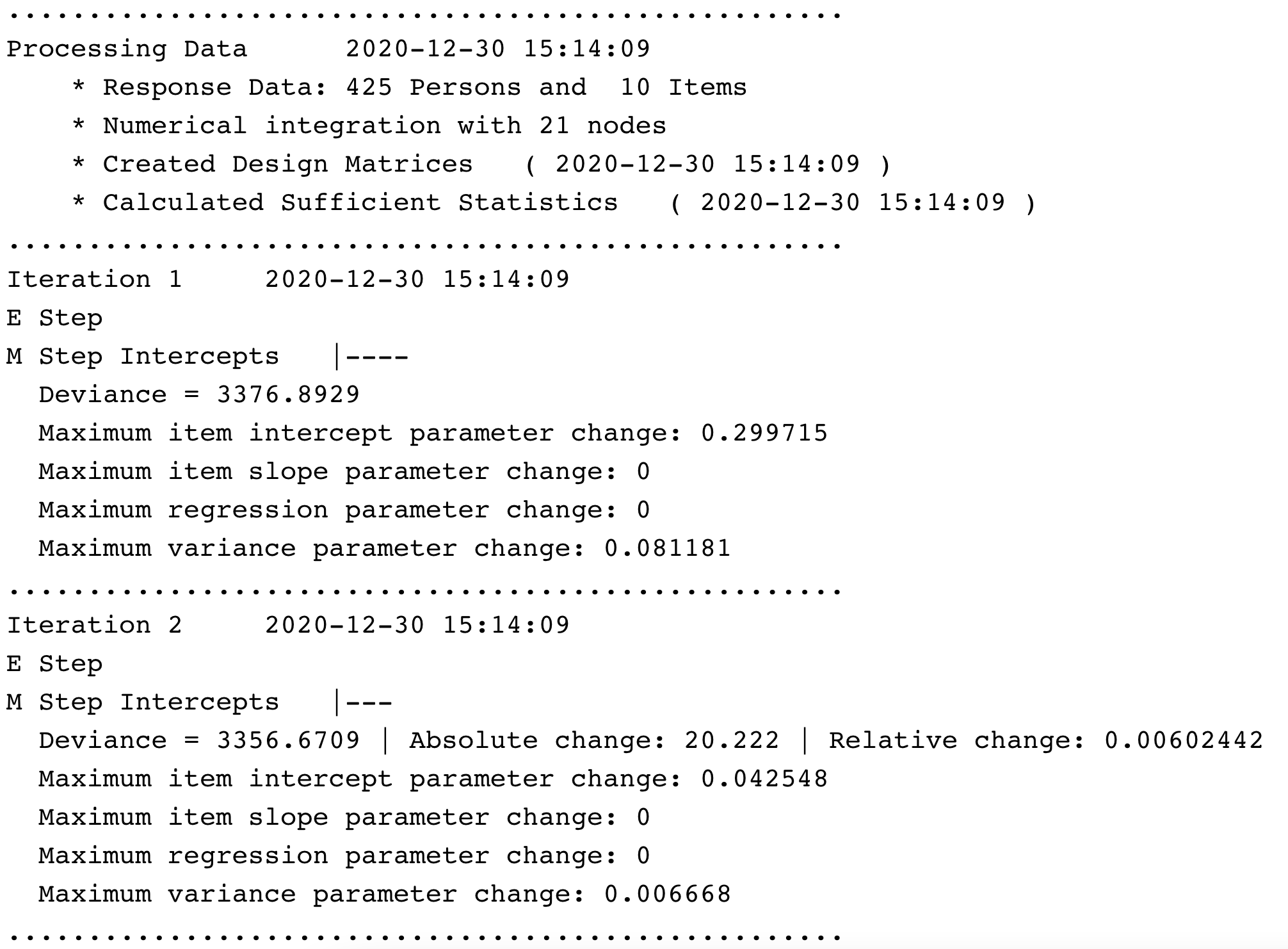
Iteration Information
After you run the tam() function, your console will show estimates of item parameters (item difficulty locations), reliability estimates, and a summary of the time in which the analysis was completed. We will explore each of these results in more detail later.
[Cheng - can we add a screenshot here?] [Dr.Wind, the tam() result do not include item estimates. The item parameters shows up when you call summary() function]
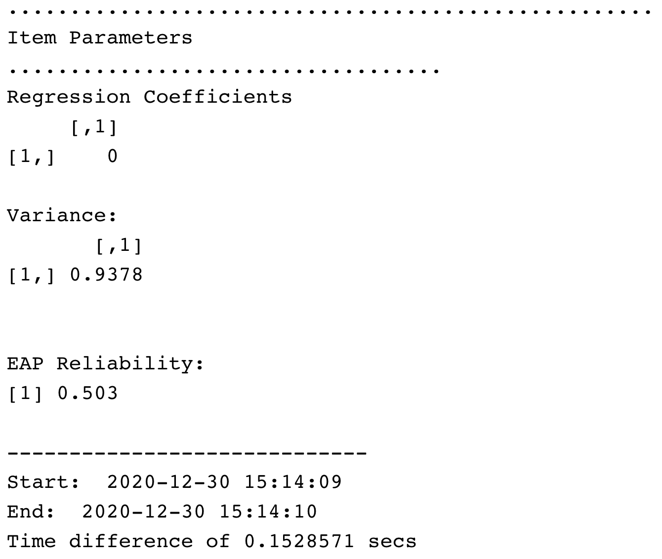
TAM Result
2.3.3 Overall Model Summary
The next step is to request a summary of the model estimation results in order to begin to understand the results from the analysis. We can do so by applying the summary() function to the model object:
## ------------------------------------------------------------
## TAM 3.5-19 (2020-05-05 22:45:39)
## R version 3.6.2 (2019-12-12) x86_64, linux-gnu | nodename=bookdown | login=unknown
##
## Date of Analysis: 2021-01-05 19:53:34
## Time difference of 0.1018295 secs
## Computation time: 0.1018295
##
## Multidimensional Item Response Model in TAM
##
## IRT Model: 1PL
## Call:
## tam.mml(resp = resp)
##
## ------------------------------------------------------------
## Number of iterations = 26
## Numeric integration with 21 integration points
##
## Deviance = 3354.91
## Log likelihood = -1677.46
## Number of persons = 425
## Number of persons used = 425
## Number of items = 10
## Number of estimated parameters = 11
##     Item threshold parameters = 10
##     Item slope parameters = 0
##     Regression parameters = 0
##     Variance/covariance parameters = 1
##
## AIC = 3377  | penalty=22    | AIC=-2*LL + 2*p
## AIC3 = 3388  | penalty=33    | AIC3=-2*LL + 3*p
## BIC = 3421  | penalty=66.57    | BIC=-2*LL + log(n)*p
## aBIC = 3386  | penalty=31.56    | aBIC=-2*LL + log((n-2)/24)*p  (adjusted BIC)
## CAIC = 3432  | penalty=77.57    | CAIC=-2*LL + [log(n)+1]*p  (consistent AIC)
## AICc = 3378  | penalty=22.64    | AICc=-2*LL + 2*p + 2*p*(p+1)/(n-p-1)  (bias corrected AIC)
## GHP = 0.39728     | GHP=( -LL + p ) / (#Persons * #Items)  (Gilula-Haberman log penalty)
##
## ------------------------------------------------------------
## EAP Reliability
## [1] 0.503
## ------------------------------------------------------------
## Covariances and Variances
##       [,1]
## [1,] 0.938
## ------------------------------------------------------------
## Correlations and Standard Deviations (in the diagonal)
##       [,1]
## [1,] 0.968
## ------------------------------------------------------------
## Regression Coefficients
##      [,1]
## [1,]    0
## ------------------------------------------------------------
## Item Parameters -A*Xsi
##       item   N     M xsi.item AXsi_.Cat1 B.Cat1.Dim1
## 1  task_01 425 0.941   -3.169     -3.169           1
## 2  task_02 425 0.809   -1.701     -1.701           1
## 3  task_03 425 0.885   -2.368     -2.368           1
## 4  task_04 425 0.784   -1.517     -1.517           1
## 5  task_05 425 0.802   -1.649     -1.649           1
## 6  task_06 425 0.974   -4.070     -4.070           1
## 7  task_07 425 0.845   -1.982     -1.982           1
## 8  task_08 425 0.967   -3.811     -3.811           1
## 9  task_09 425 0.301    1.002      1.002           1
## 10 task_10 425 0.520   -0.093     -0.093           1
##
## Item Parameters in IRT parameterization
##       item alpha   beta
## 1  task_01     1 -3.169
## 2  task_02     1 -1.701
## 3  task_03     1 -2.368
## 4  task_04     1 -1.517
## 5  task_05     1 -1.649
## 6  task_06     1 -4.070
## 7  task_07     1 -1.982
## 8  task_08     1 -3.811
## 9  task_09     1  1.002
## 10 task_10     1 -0.093
From these results, we suggest taking a quick look at the Item Parameters as reported in the table labeled Item Parameters in IRT parameterization.
[Cheng - can we add a screenshot here?]
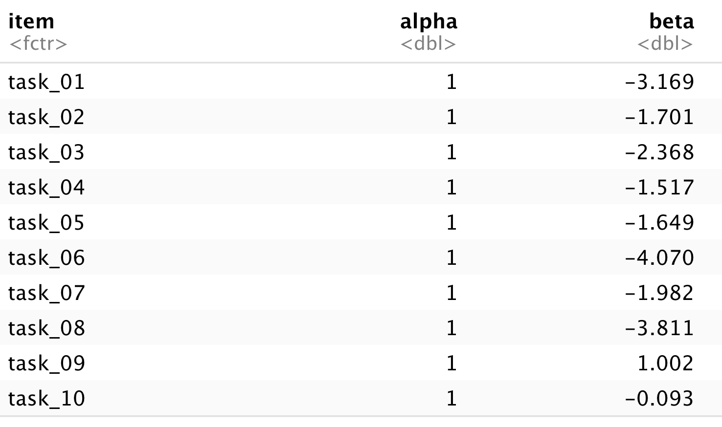
Because we ran a Rasch model, the alpha (discrimination) parameters are fixed to a constant value of 1. The beta parameters are the item locations on the latent variable. We will explore the item locations in more detail later in the analysis.
2.3.4 Plot a Wright Map to visualize item and person locations:
A useful feature of Rasch models is that when there is acceptable fit between the model and the data (discussed in detail in in Chapter 3), it is possible to visualize and compare item and person locations on a single linear continuum. Professor Bejamin D. Wright popularized an approach to displaying Rasch model results on a linear continuum, and this technique has been widely adopted by Rasch measurement researchers across disciplines. In his honor, these displays are often called Wright Maps. In the literature, researchers also refer to these displays as Variable Maps. Please see Wilson (2011) for a discussion of the term Wright Map.
As the next step in our analysis, we will use the WrightMap package to create a Wright Map from our model results. We will create the plot using the function IRT.WrightMap() on the model object (dichot.transreas). We will set the option for displaying threshold labels as FALSE, because we are working with dichotomous data. We also used the main.title= option to customize the title of the plot.
# Plot the Wright Map
IRT.WrightMap(dichot.transreas, show.thr.lab=FALSE, main.title = "Transitive Reasoning Wright Map")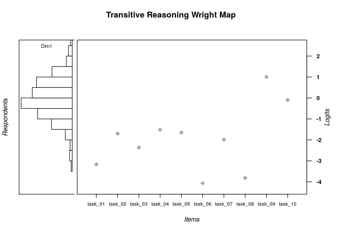 In this Wright Map display, the results from the dichotomous Rasch model analysis of the transitive reasoning data are summarized grapihcally. The figure is organized as follows:
The left panel of the plot shows a histogram of respondent (person) locations on the logit scale that represents the latent variable. Units on the logit scale are shown on the far-right axis of the plot (labeled Logits). In the panel with the person locations, the label “Dim1” means that the distribution of person locations is specific to one dimension. In multi-dimensional Rasch model (Brigs & Wilson, 2003) and multidimensional IRT analyses (Bonifay, 2019; Reckase, 2009), the Wright Map can show multiple distributions of person locations that correspond to each dimension in the model.
[Cheng - can we add a screenshot here with an arrow pointing to the left panel of the Wright map?]
[Dr. Wind, do you think put two arrows in one map might be better?]
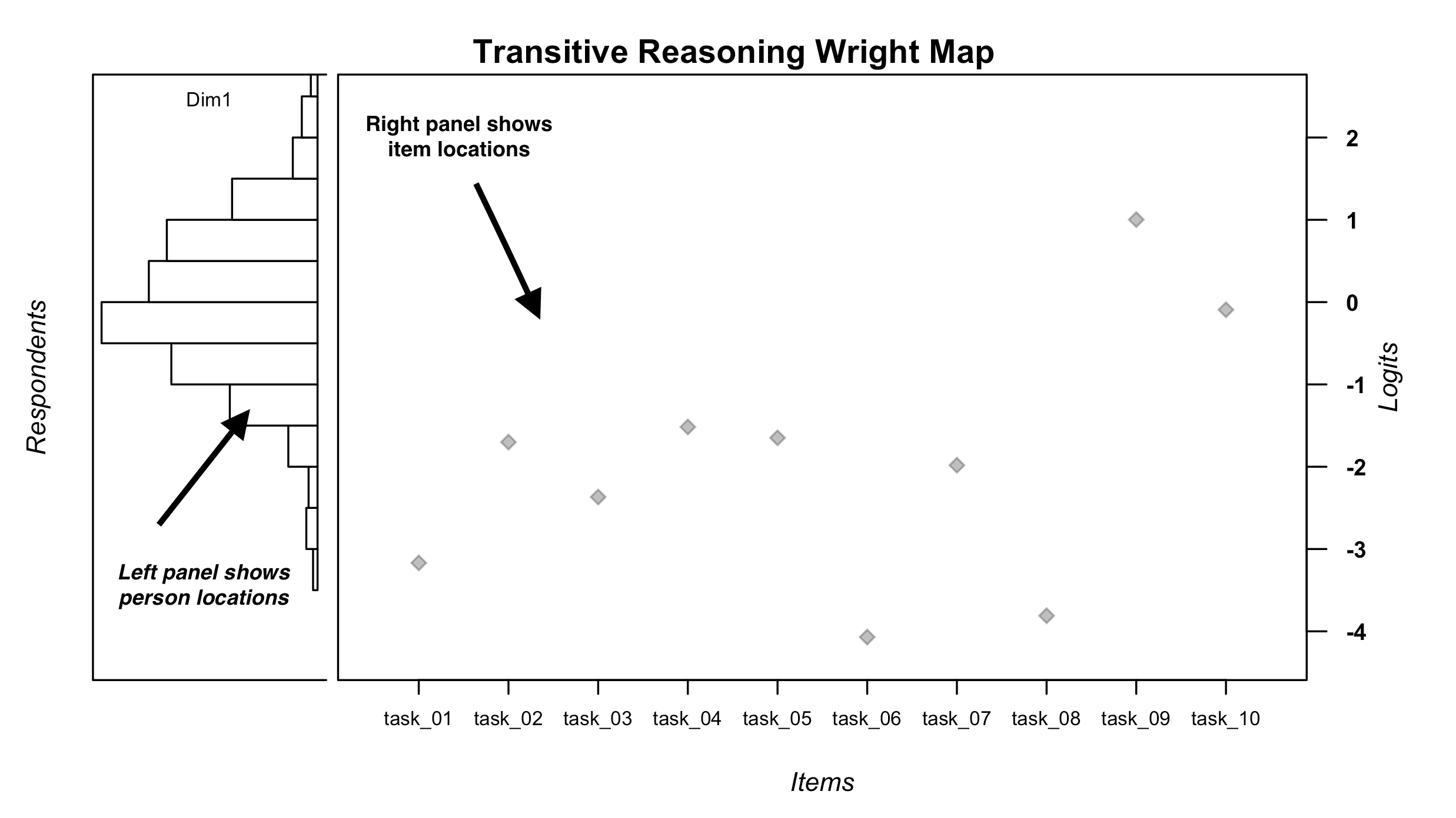
The large central panel of the plot shows the item locations (item difficulty estimates) on the logit scale that represents the latent variable. Light grey diamond shapes show the logit scale location of each item, as labeled on the x-axis.
[Cheng - can we add a screenshot here with an arrow pointing to the central panel of the Wright map?] [Dr.Wind, If you want to divide the previous Map for a better illustration, I can also do that.]
Even though it is not appropriate to fully interpret item and person locations on the logit scale until there is evidence of acceptable model-data fit, we recommend examining the Wright Map during the preliminary stages of an item analysis to get a general sense of the model results and to identify any potential scoring or data entry errors.
A quick glance at the Wright Map suggests that, on average, the persons are located higher on the logit scale compared to the average item locations. In addition, there appears to be a relatively wide spread of person and item locations on the logit scale, such that the transitive reasoning test appears to be a useful tool for identifying differences in person locations and item locations on the latent variable. We will return to this display for more exploration after checking for acceptable model-data fit, among other psychometric properties.
2.3.5 Examine Item Parameters:
As the next step in our analysis, we will examine the item parameters in detail. We will use the $ operator to request the item location esitmates (xsi) from the dichot.transreas object and store the results in a new object called difficulty:
By running this code, we have created a dataframe object that includes two variables: item difficulty estimates labeled xsi, and standard errors labeled se.xsi. The row labels show the item names from our response matrix.
Because this example dataset only includes 10 items, we can quickly examine the results by printing the difficulty object to the R console as follows:
##                 xsi    se.xsi
## task_01 -3.16864785 0.2133573
## task_02 -1.70089350 0.1321453
## task_03 -2.36782604 0.1600094
## task_04 -1.51715819 0.1265292
## task_05 -1.64916897 0.1304829
## task_06 -4.06989050 0.3113083
## task_07 -1.98241949 0.1423829
## task_08 -3.81092249 0.2780165
## task_09  1.00240165 0.1145384
## task_10 -0.09324812 0.1061752
Alternatively, we can examine the dataframe by clicking on it in the Environment pane of R Studio or by using the View() function with the difficulty object: