10 Correlation
In our chapter 7, we introduced descriptive statistics; mean, variance, median, kurtosis, etc. These descriptive statistics aimed to ease the communication for a single variable. In other words, instead of transferring the entire raw data set to a colleague (or to a machine), providing these descriptives is generally satisfying and easier. However when the interest is in the association between variables, other measures are needed.
The sum of cross products, \(S_{XY}=\sum(X-\bar X)(Y- \bar Y)\), can provide some information about the association. For example Figure 10.1 depicts an X and a Y variable. The sum of cross products for these two variables is zero.
##        x     y deviationX deviationY crossPRODUCT
## 1   1.00  0.00       0.93       0.00         0.00
## 2   0.90  0.43       0.83       0.43         0.36
## 3   0.62  0.78       0.56       0.78         0.44
## 4   0.22  0.97       0.16       0.97         0.15
## 5  -0.22  0.97      -0.29       0.97        -0.28
## 6  -0.62  0.78      -0.69       0.78        -0.54
## 7  -0.90  0.43      -0.97       0.43        -0.42
## 8  -1.00  0.00      -1.07       0.00         0.00
## 9  -0.90 -0.43      -0.97      -0.43         0.42
## 10 -0.62 -0.78      -0.69      -0.78         0.54
## 11 -0.22 -0.97      -0.29      -0.97         0.28
## 12  0.22 -0.97       0.16      -0.97        -0.15
## 13  0.62 -0.78       0.56      -0.78        -0.44
## 14  0.90 -0.43       0.83      -0.43        -0.36
## 15  1.00  0.00       0.93       0.00         0.00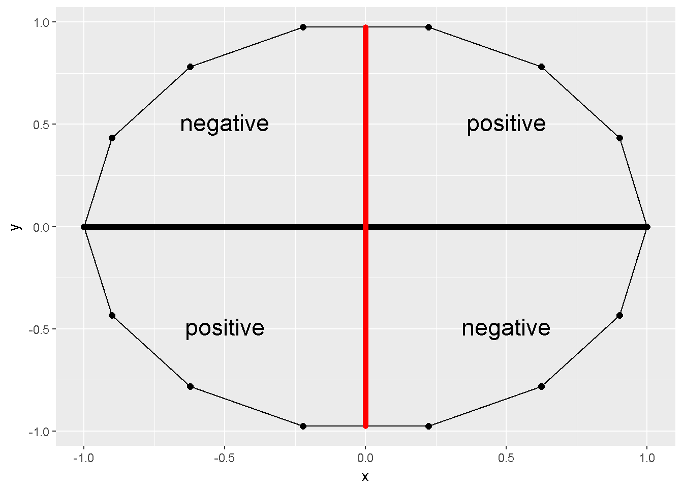
Figure 10.1: Sum of cross products=0
The covariance between two variable is simply \(Cov_{XY}=S_{XY}/n-1\), but its a scale dependent measure, the correlation coefficient on the other hand generally has its bounds.
10.1 Pearson correlation coefficient
Pearson introduced a correlation coefficient in 1896. This coefficient ranges between -1 and +1, can be calculated as \(Cov_{XY}/S_X S_Y\). This coefficient measures the linear relationship between two variables. Figure 10.1 depicts a correlation of zero. Even though X and Y in this figure are related to form a 14-sided polygon, the relation is not linear. Hence the correlation is zero. Figure 10.2 depicts several other associations; (A) is a perfect positive linear relationship, (B)is a positive correlation of .7, (C) substantially no linear relation, (D) is a correlation of -.4 and (E) is a correlation of -1.
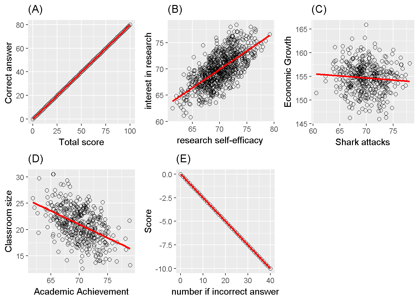
Figure 10.2: Correlation examples
10.1.1 Inference on a Pearson correlation coefficient
Information from the sample (\(r\)) can be utilized to make judgement about the population (\(\rho\)).
The z transformation , assuming a bivariate normality and a sample size of at least 10 (Myers et al. (2013)), is a helpful procedure to reach a judgement. The transformation equation is; \[z_r = \frac{1}{2}ln \left( \frac{1+r}{1-r} \right)\]
The standard error is; \[\sigma_r = \frac{1}{\sqrt{n-3}}\]
Hence the confidence intervals are \(z_r \pm z_{\alpha / 2} \sigma_r\). Back transformation is needed to make interpretation about the correlation coefficient; \(r=\frac{e^{2z_r}-1}{e^{2z_r}+1}\).
Utilizing a normal distribution, a null hypothesis can be tested; \[z=\frac{z_r - z_{\rho_{null}}}{\frac{1}{\sqrt{n-3}}}\] The t distribution can also be utilized to test \(H_0:\rho=0\).
\[t=r\sqrt{\frac{n-2}{1-r^2}}\]
The distribution for this statistic follows a t distribution with a degrees of freedom of \(n-2\).
10.1.2 R codes for Pearson Correlation coefficent
For illustrative purposes we selected the city of Bayburt. The Pearson correlation is computed for the association between the Gender Attitudes scores and the annual income per person. The income per person is calculated as “total household income” divided by the “total number of residents in the house”.
# load csv from an online repository
urlfile='https://raw.githubusercontent.com/burakaydin/materyaller/gh-pages/ARPASS/dataWBT.csv'
dataWBT=read.csv(urlfile)

#remove URL
rm(urlfile)

#select the city of Bayburt
# listwise deletion for gen_att and education variables
dataWBT_Bayburt=dataWBT[dataWBT$city=="BAYBURT",]
#hist(dataWBT_Bayburt$income_per_member)
The bivariate distribution can be seen in 10.3. This is an interactive graph, please use your mouse to inspect it, created with the rgl package (Adler and Murdoch (2017)).
## wgl
##   1
Figure 10.3: Gender Attitudes and Income
Bivariate normality seems to be violated. For comparison, below graph 10.4.depicts a bivariate normal distribution with r=0.7. Nevertheless, for illustrative purposes we use these data to test the null hypothesis \(H_0: \rho=0\) against the non-directional alternative hypothesis \(H_1: \rho \neq0\).The scatter plot is provided in 10.5.
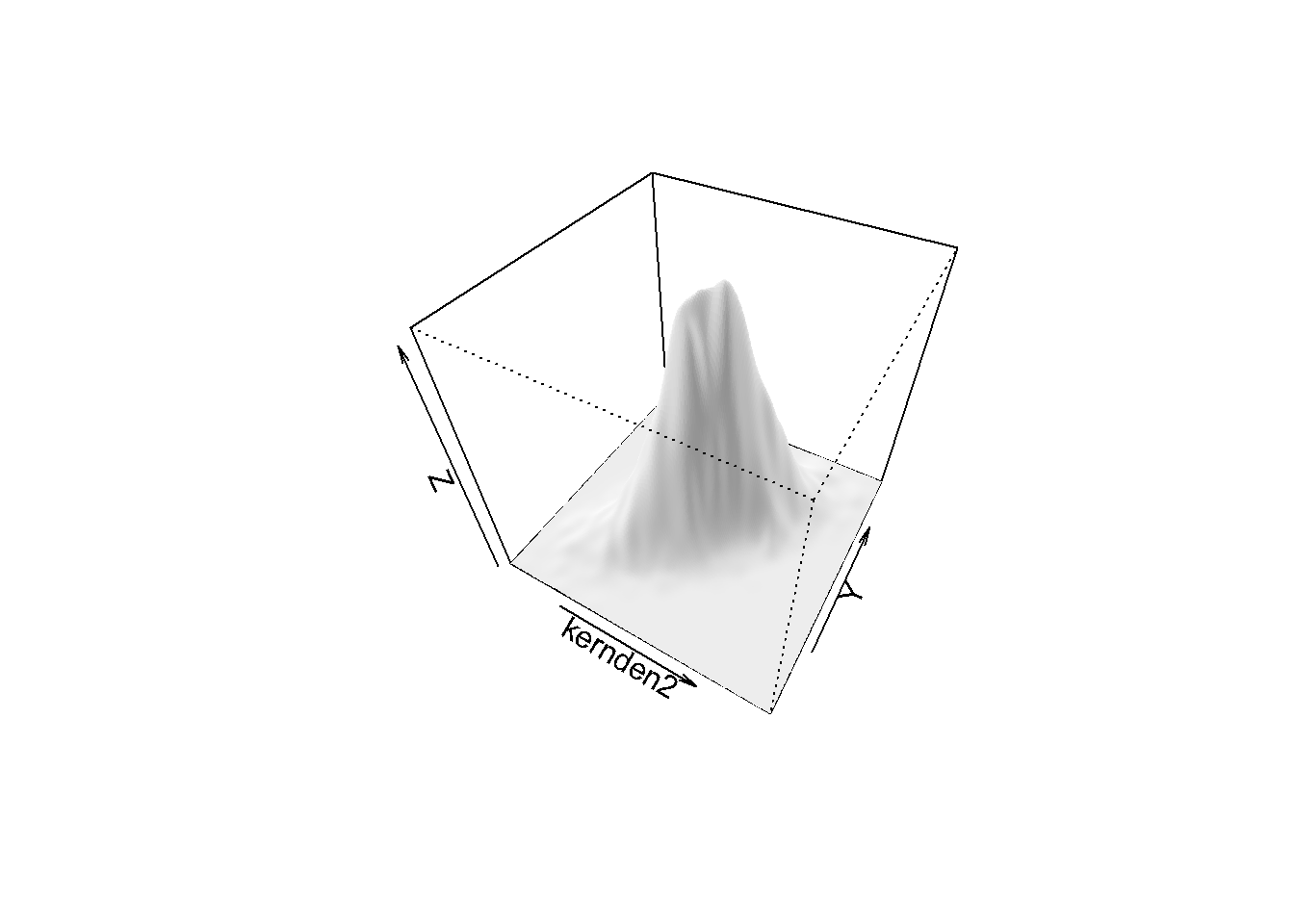
Figure 10.4: Bivariate Normal Distribution
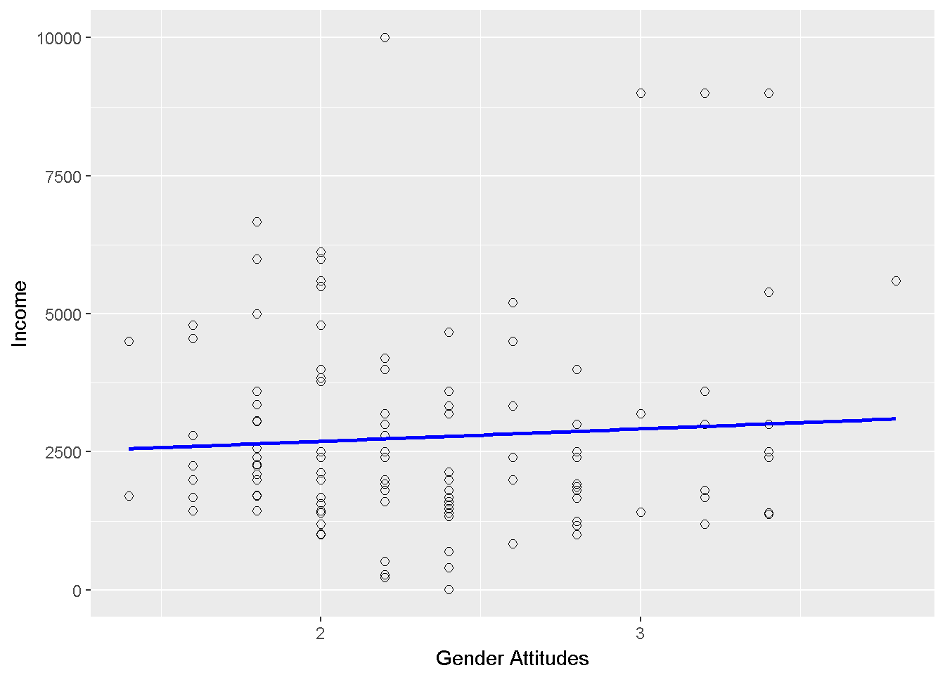
Figure 10.5: Bayburt: Gender attitudes vs income scatterplot
The correlation between these two variables is computed by the cor function in the stats package (R Core Team (2016b)). The cor.test function in the same package performs the t-test and provides a confidence interval based on Fisher’s z transformation.
#use ?cor to see use="complete.obs" is doing casewise deletion

with(dataWBT_Bayburt,cor(gen_att,income_per_member,
                         use = "complete.obs",method="pearson"))
## [1] 0.0664

with(dataWBT_Bayburt,cor.test(gen_att,income_per_member,
         alternative = "two.sided",
         method="pearson",
         conf.level = 0.95,
         na.action="na.omit"))
##
##  Pearson's product-moment correlation
##
## data:  gen_att and income_per_member
## t = 0.8, df = 100, p-value = 0.4
## alternative hypothesis: true correlation is not equal to 0
## 95 percent confidence interval:
##  -0.102  0.232
## sample estimates:
##    cor
## 0.0664
These procedures can easily be hard coded.Stating \(H_0: \rho=0\) and \(H_0: \rho \neq 0\)
sample_r=0.06641641
r0=0        #the null
sample_n=137       # the number of complete.cases
zr=(0.5)*log((1+sample_r)/(1-sample_r))  # Z transformasyonu
z0=(0.5)*log((1+r0)/(1-r0))  # Z transformasyonu
sigmar=1/(sqrt(sample_n-3))

#the z test statistic
(zr-z0)/sigmar
## [1] 0.77


ll=zr-(qnorm(0.975)*sigmar)  # lower limit


ul=zr+(qnorm(0.975)*sigmar)  # upper limit


(exp(2*ll)-1)/(exp(2*ll)+1)  #transformback
## [1] -0.102
(exp(2*ul)-1)/(exp(2*ul)+1)  #transformback
## [1] 0.232


t=sample_r*(sqrt((sample_n-2)/(1-sample_r^2)))
qt(c(.025, .975), df=(sample_n-2))
## [1] -1.98  1.98
p.value = 2*pt(-abs(t), df=sample_n-2)
p.value
## [1] 0.441
A percentile bootstrap method might perform satisfactorily as a robust approach (Myers et al. (2013))
#Calculate 95% CI using bootstrap (normality is not assumed)
set.seed(31012017)
B=5000       # number of bootstraps
alpha=0.05   # alpha

#gender attitudes and income
originaldata=dataWBT_Bayburt2

#add id
originaldata$id=1:nrow(originaldata)

output=c()
for (i in 1:B){
  #sample rows
  bs_rows=sample(originaldata$id,replace=T,size=nrow(originaldata))
  bs_sample=originaldata[bs_rows,]
  output[i]=cor(bs_sample$gen_att,bs_sample$income_per_member)
  }
output=sort(output)

## Non-directional
# lower limit
output[as.integer(B*alpha/2)]
## [1] -0.138

# d star upper
output[B-as.integer(B*alpha/2)+1]
## [1] 0.252
There are alternatives to percentile bootstrapping for a correlation coefficient, extensively discussed by Wilcox (2012). The WRS 2 package offers two alternatives, the percentage bend correlation and the Winsorized correlation. Only for illustrative purposes below is an R code;
# investigate the WRS package
library(WRS2)
pbcor(dataWBT_Bayburt2$gen_att,dataWBT_Bayburt2$income_per_member,beta=.2)
## Call:
## pbcor(x = dataWBT_Bayburt2$gen_att, y = dataWBT_Bayburt2$income_per_member,
##     beta = 0.2)
##
## Robust correlation coefficient: -0.0351
## Test statistic: -0.407
## p-value: 0.684

wincor(dataWBT_Bayburt2$gen_att,dataWBT_Bayburt2$income_per_member,tr=.2)
## Call:
## wincor(x = dataWBT_Bayburt2$gen_att, y = dataWBT_Bayburt2$income_per_member,
##     tr = 0.2)
##
## Robust correlation coefficient: -0.0197
## Test statistic: -0.229
## p-value: 0.82
Write up: We tested a null hypothesis stating the gender attitudes scores and income variable are correlated against an non-directional alternative hypothesis. The Pearson correlation coefficient was \(r=.066,p=.44\), the confidence interval with a .05 probability of a type I error using the z transformation is -.10 to .23. The null hypothesis is retained. This conclusion is consistent with the bootstrap results, using 5000 iterations, the 95% CI is -.138 to .252.
Sign difference note The Pearson correlation coefficent is .066 but not significantly different than zero. The WRS package functions also agreed to retain the null but the coefficent was negative. The income variable was slightly skewed due to a small number of relatively large income values. In fact, when the World Bank team analyzed the data using a regression, they top-coded and transformed the income variable (for details Hirshleifer et al. (2016)). Let us top-code and transform the income variable, inspect bivariate normality and calculate the Pearson correlation;
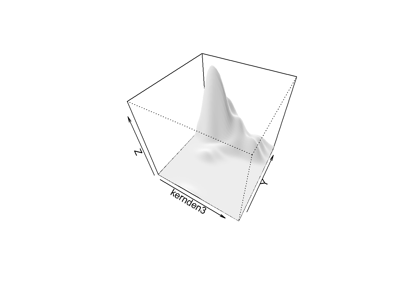
Figure 10.6: Top-coded and transformed income variable
with(dataWBT_Bayburt2,cor.test(gen_att,incomeTC,
         alternative = "two.sided",
         method="pearson",
         conf.level = 0.95,
         na.action="na.omit"))
##
##  Pearson's product-moment correlation
##
## data:  gen_att and incomeTC
## t = -0.009, df = 100, p-value = 1
## alternative hypothesis: true correlation is not equal to 0
## 95 percent confidence interval:
##  -0.169  0.167
## sample estimates:
##      cor
## -0.00081
Top-coding and transforming the income variable produced a distribution relatively closer to normal. The sign of the Pearson correlation coefficent is negative.
10.2 Spearman’s rho and Kendall’s tau
When the data is in the rank format, or there is a need for protection against outliers15 when working with continuous data the Spearman correlation coefficient is used. If the number of ties in the ranks is not large, procedures provided for the Pearson correlation coefficient can be utilized. Setting the method argument to “spearman”, the cor.test function first transforms the data into ranks and performs the procedures introduced for the Pearson coefficient.
10.2.1 The R code for Spearman’s rho and Kendall’s tau
We calculated the Pearson correlation coefficient to assess the association between the gender attitudes scores and the income for the participants in Bayburt. The Spearman correlation coefficient can conveniently be calculated by R;
#use ?cor to see use="complete.obs" is doing casewise deletion
with(dataWBT_Bayburt,cor.test(gen_att,income_per_member,
         alternative = "two.sided",
         method="spearman",
         conf.level = 0.95,
         na.action="na.omit",
         exact=FALSE))
##
##  Spearman's rank correlation rho
##
## data:  gen_att and income_per_member
## S = 5e+05, p-value = 0.6
## alternative hypothesis: true rho is not equal to 0
## sample estimates:
##     rho
## -0.0508
When there are ties, the cor.test function corrects the Spearman coefficient but the exact p value can not be calculated. Instead exact=FALSE argument yields a p value based on a t distribution. Field, Miles, and Field (2012) suggests using Kendall’s tau with large number of ties;
#use ?cor to see use="complete.obs" is doing casewise deletion
with(dataWBT_Bayburt,cor.test(gen_att,income_per_member,
         alternative = "two.sided",
         method="kendall",
         conf.level = 0.95,
         na.action="na.omit",
         exact=FALSE))
##
##  Kendall's rank correlation tau
##
## data:  gen_att and income_per_member
## z = -0.6, p-value = 0.5
## alternative hypothesis: true tau is not equal to 0
## sample estimates:
##     tau
## -0.0373
The exact=FALSE argument with method=“kendall” uses normal approximation.
The Spearman correlation between the gender attitudes scores and income was \(r_S=-.051, p=.56\), and the Kendall’s tau was \(\tau = -.037,p=.54\)
10.3 Biserial and Point-Biserial Correlation Coefficients with R
The association between a continuous variable and a dichotomously reflected latent continuous variable can be examined with a biserial correlation. In psychometrics , for example, biserial correlation is used for calculating the correlation between a total test score (continuous) and a dichotomous item score (assumed to underlie a latent variable).
For illustrative purposes let us use dichotomized item116 and the gender attitudes score. The biserial function in the psych (Revelle (2016)) package can calculate the bi-serial correlation;
dataWBT_Bayburt$binitem1=ifelse(dataWBT_Bayburt$item1==4,1,0)
require(psych)
with(dataWBT_Bayburt,biserial(gen_att,binitem1))
##       [,1]
## [1,] 0.317
The point-biserial correlation is calculated for an association between a dichotomous variable and a continuous variable. The cor.test function with method=“pearson” can be used to calculate a point-biserial correlation. The association between the gender and the gender attitudes scores is examined below;
dataWBT_Kayseri=dataWBT[dataWBT$city=="KAYSERI",]
dataWBT_Kayseri$genderNUM=ifelse(dataWBT_Kayseri$gender=="Female",1,0)
with(dataWBT_Kayseri,cor.test(gen_att,genderNUM,
         alternative = "two.sided",
         method="pearson",
         conf.level = 0.95,
         na.action="na.omit"))
##
##  Pearson's product-moment correlation
##
## data:  gen_att and genderNUM
## t = -7, df = 200, p-value = 2e-10
## alternative hypothesis: true correlation is not equal to 0
## 95 percent confidence interval:
##  -0.487 -0.277
## sample estimates:
##    cor
## -0.387
10.4 Phi Correlation Coefficient with R
When the two variables are dichotomous, a phi (\(\phi\)) correlation coefficient is calculated. For illustrative purposes we calculated the phi coefficent between the gender and the wage variable. This variable equals to “yes” if one of the house members receives wage in the past 12 months. The phi function in the psych package requires the 2 x 2 matrix of frequencies to calculate the phi coefficient.
dataWBT_Kayseri=dataWBT[dataWBT$city=="KAYSERI",]
table(dataWBT_Kayseri$gender,dataWBT_Kayseri$wage01)
##
##           No Yes
##   Female  52  97
##   Male    49  54
##   Unknown  0   0

genderWAGE=matrix(c(52,49,97,54),ncol=2)
library(psych)
phi(genderWAGE)
## [1] -0.13

phi(genderWAGE)
## [1] -0.13
10.5 Tetrachoric and Polychoric Correlation Coefficients with R
When the two variables are dichotomous but their underlying distributions are assumed to be bivariate normal, a tetrachoric correlation (rt) is calculated. For example students` answers on an achievement test, if coded as 1 for correct and 0 otherwise, can be considered as dichotomous variables with underlying normal distributions and the linear relationship between these underlying distributions can be estimated with a tetrachoric correlation coefficient. For illustrative purposes, let us use dichotomized item3 and item6 . The tetrachoric function in the psych (Revelle, 2016) package can calculate the tetrachoric correlation, and in our case it is found to be .07;
# items 3. and 6. Are dichotomized
dataWBT_Kayseri$Bitem3=ifelse(dataWBT_Kayseri$item3==1|dataWBT_Kayseri$item3==2,1,0)
dataWBT_Kayseri$Bitem6=ifelse(dataWBT_Kayseri$item6==1|dataWBT_Kayseri$item6==2,1,0)
require(psych)
tetrachoric(as.matrix(dataWBT_Kayseri[,c("Bitem3","Bitem6")]))
## Call: tetrachoric(x = as.matrix(dataWBT_Kayseri[, c("Bitem3", "Bitem6")]))
## tetrachoric correlation
##        Bitm3 Bitm6
## Bitem3 1.00
## Bitem6 0.07  1.00
##
##  with tau of
## Bitem3 Bitem6
##  -0.23   0.54
When the two variables are ordered categorical but their underlying distributions are assumed to be continiuos, a polychoric correlation coefficient is calculated. For example participants` answers for Likert type questions are generally considered as ordinal variables. Uebersax (2015) uses the term ‘latent continuous correlations’ both for tetrachoric and polychoric correlations. There are at least two frameworks to calculate latent continuous correlations, closed forms or iterative procedures. Readers are referred to Olsson (1979) and to technical details of the polychoric function in the psych package. We also suggest researchers to provide details of the software they use when calculating a latent continiuos correlation, when using R the default settings should be studied carefully. For illustrative purposes let us use item3 and item6. These two variables were created using a 4-point Likert scale. The polychoric correlation between these two items is found to be .16;
require(psych)
polychoric(as.matrix(dataWBT_Kayseri[,c("item3","item6")]))
## Call: polychoric(x = as.matrix(dataWBT_Kayseri[, c("item3", "item6")]))
## Polychoric correlations
##       item3 item6
## item3 1.00
## item6 0.16  1.00
##
##  with tau of
##           1     2    3
## item3 -0.72  0.23 1.30
## item6 -1.37 -0.54 0.82
10.6 Issues in Interpreting Correlation Coefficients
Several issues arise in interpreting correlation coefficients.
Causation A correlation coefficient does not imply causation. For any correlation there are at least four possible interpretations involving causation: (a) X causes Y, (b) Y causes X, (c) both X and Y share one or more common causes, and (d) X and Y have different causes, but these causes are correlated.
The magnitude Whether a correlation of .6 is large or not depends on the context. For example suppose the .6 is the correlation between scores on two forms of a standardized achievement tests. This correlation is called an alternate forms reliability coefficient. Alternate forms reliability coefficients for standardized tests are expected to be at least .70 and preferably higher, so the .6 correlation would be regarded as small. Now suppose the correlation is between GRE scores and GPA. The correlation between GRE scores and GPA is typically somewhere between .10 and .30, so a .60 correlation would be a very large correlation coefficient.
Outliers Correlation coefficients can be misleading when the data set contains outliers.
Reliability If either X or Y contains measurement error, the effect of the measurement error is to attenuate the correlation coefficient. Attenuate means to make the correlation coefficient closer to zero than it would have been if there had been no measurement error.
It is possible to correct for attenuation using \[r_{T_x T_y}=\frac{r_{xy}}{\sqrt(r_{xx}r_{yy})}\] where \(r_{xx}\) and \(r_{yy}\) are the reliability coefficients.
• When NOT to correct for attenuation: When a variable is used for practical decision making and we are interested in the validity of those decisions, we should NOT correct for attenuation because the decisions are made on the basis of an observed variable, not a true variable.
• When to correct for attenuation: We can correct for attenuation when our motivation is to examine theory.
• Comparison of Correlation Coefficients: A comparison of correlation coefficients for two variables with a third variable can be affected by differences in reliability for the first two variables. If we are interested in theoretical relationships between variables and we want to compare the strength of relationship of two constructs (call these A and B and let them be measured by X1 and X2 ) with a third (call this C and let it be measured by Y), the comparison of the strength of relationship between A and C to the strength of relationship between B and C is compromised if X1 and X2 have different reliability coefficients. To compare strength of relationship we want the reliability of X1 and X2 to be the similar. Of course, it is best if both reliability coefficients are high, but it is critical that they are quite similar.
Unit of analysis A correlation calculated for one unit of analysis (e.g., individuals without regard to school) should not be applied to other units of analysis (i.e., individuals within schools or school means).
Variance in the two variables being correlated The correlation coefficient for two variables can be strongly affected by the amount of variance for the variables being correlated. Other things being equal when the variance of either or both variables is small, the correlation will tend to be small. If the variance for either or both variables is artificially small, misleading small correlation coefficients can occur. Variance can be artificially small due to
• Categorizing Based on Quantitative Variables
• Limited Range Scales
• Restriction of range
• Floor and Ceiling Effects
References
Myers, Jerome L., A. Well, Robert F. Lorch, and Ebooks Corporation. 2013. Research Design and Statistical Analysis. 3rd ed. New York: Routledge.
Adler, Daniel, and Duncan Murdoch. 2017. Rgl: 3D Visualization Using Opengl. https://CRAN.R-project.org/package=rgl.
R Core Team. 2016b. R: A Language and Environment for Statistical Computing. Vienna, Austria: R Foundation for Statistical Computing. https://www.R-project.org/.
Wilcox, Rand R. 2012. Introduction to Robust Estimation and Hypothesis Testing. 3rd;3; US: Academic Press.
Hirshleifer, Sarojini, David McKenzie, Rita Almeida, and Cristobal Ridao-Cano. 2016. “The Impact of Vocational Training for the Unemployed: Experimental Evidence from Turkey.” The Economic Journal 126 (597): 2115–46.
Field, Andy P., Jeremy Miles, and Zoë Field. 2012. Discovering Statistics Using R. Thousand Oaks, Calif;London; Sage.
Revelle, William. 2016. Psych: Procedures for Psychological, Psychometric, and Personality Research. https://CRAN.R-project.org/package=psych.
Uebersax, John S. 2015. “Introduction to the Tetrachoric and Polychoric Correlation Coefficients.” Obtenido de Http://Www. John-Uebersax. Com/Stat/Tetra. Htm.[Links].
Olsson, Ulf. 1979. “Maximum Likelihood Estimation of the Polychoric Correlation Coefficient.” Psychometrika 44 (4). Springer: 443–60.