9 Analysis of Variance (ANOVA)
9.1 Terminology
Designs are usually described using a standard terminology. The following is an introduction to this terminology.
Factor a collection of treatments. For example, in the Magnetic vs. Inactive device study, device is a factor. In the priming study, type of prime word is a factor.
Level an instance of a factor. In the Magnetic vs. Inactive device study 8.3.2, magnetic device is a level of the type of instruction factor, as is inactive device. In the priming study, weapon word is a level of the type of prime word factor, as is non-weapon word.
Crossed factors two factors are crossed if each level of one factor occurs in combination with every level of the second factor. For example, consider the diagram of a repeated measures design in which the treatment factor has two levels.
| Levels of Treatment Factor | ||
|---|---|---|
| 1 | 2 | |
| Subjects | ||
| 1 | ||
| 2 | ||
| . | ||
| n |
Subjects can be considered a factor and are crossed with the treatment factor since each subject occurs in combination with each treatment.
Nesting one factor is nested in a second factor if each level of the first factor occurs in combination with only one level of the second factor. For example, consider the following diagram of an independent samples design in which the treatment factor has two levels.
| Levels of Treatment Factor | |
|---|---|
| 1 | 2 |
| \(S_1\) | \(S_{n+1}\) |
| \(S_2\) | \(S_{n+2}\) |
| \(S_3\) | \(S_{n+3}\) |
| … | |
| \(S_n\) | \(S_{2n}\) |
Subjects are nested in treatments because each subject appears in only one treatment.
Within-subjects factor a factor that is crossed with subjects. The name derives from the fact that the levels of the factor vary within a subject as can be seen in the diagram for the repeated measures design. The following designs have a within-subjects factor: subjects as own control and longitudinal, both of which are examples of repeated measures designs.
Within-blocks factor a factor that is crossed with blocks. The name derives from the fact that the levels of the factor vary within a block as can be seen in the following diagram.
| Block | Levels of factor | |
|---|---|---|
| 1 | 2 | |
| 1 | ||
| 2 | ||
| … | ||
| n |
The following designs have a within-blocks factor: randomized block, nonrandomized block, familial, and dyads.
Many people do not distinguish between within-subjects and within-blocks factors, because they lead to the same method of analysis. Typically, we will not distinguish between the two types of factors and will label both as a within-subjects factor.
Between-subjects factor a factor that has subjects nested in its levels; the subjects in the levels are not crossed with blocks. The qualifier following the semi-colon is necessary to distinguish a between-subjects factor from a within-blocks factor because in both factors a subject is assigned to only one level of a factor. This can be seen from the diagram for the independent samples design:
| Levels of Treatment Factor | |
|---|---|
| 1 | 2 |
| \(S_1\) | \(S_{n+1}\) |
| \(S_2\) | \(S_{n+2}\) |
| \(S_3\) | \(S_{n+3}\) |
| … | |
| \(S_n\) | \(S_{2n}\) |
9.2 Between Subjects ANOVA
The name between-subjects derives from the fact that the levels of the factor vary between subjects.
9.2.1 One-way Between Subjects ANOVA
The structural model for a one-factor between subjects ANOVA is \(Y_{ij}=\mu+\alpha_{j}+\epsilon_{ij}\), in which \(Y_{ij}\) is the score for the participant i in group j, \(\mu\) is the grand mean of the scores, \(\alpha_j\) is the effect of the level j, and \(\epsilon_{ij}\) is the error term (nuisance). It can be shown that \(\mu_j=\mu+\alpha_j\), where \(\mu_j\) is the the mean for the jth level of the factor.
Generally, the interest is on \(\alpha_j\) because it represents \(\mu_j-\mu\). This interest leads to hypothesis testing: \(H_0: \mu_1 = \mu_2 = \cdots = \mu_j\)
The alternative hypothesis states that at least one population mean is different. It is possible to test the null by partitioning the variance, for a one factor model using the notation by Myers et al. (2013)
| SV | df | SS | MS | F |
|---|---|---|---|---|
| Total | \(N-1\) | \(\sum_{j=1}^{J}\sum_{i=1}^{n_j}(Y_{ij} - \bar{Y}_{\cdot \cdot})^2\) | ||
| A | \(J-1\) | \(\sum_{j=1}^{J}n_j(\bar{Y}_{\cdot j}-\bar{Y{\cdot \cdot}})^2\) | \(SS_A/df_{A}\) | \(MS_A/MS_{S/A}\) |
| S/A | \(N-J\) | \(\sum_{j=1}^{J}\sum_{i=1}^{n_j}(Y_{ij} - \bar{Y}_{\cdot j})^2\) | \(SS_{S/A} / df_{S/A}\) |
| SV | EMS |
|---|---|
| Total | |
| A | \(\sigma_{S/A}^2 + \frac{1}{J-1} \sum_{j} n_j (\mu_j-\mu)^2\) |
| S/A | \(\sigma_{S/A}^2\) |
where SV=Source of Variance, df=degrees of freedom, SS=Sum of squares, MS= Mean Square, EMS= Expected Mean Square, A is the between subjects factor with J levels, S/A is the subjects within A, N is the total sample size, j=1,…,J factor level indicator, i=1,…,\(n_j\) is the individual indicator, \(Y_{ij}\) is the individual score, \(\bar{Y}_{\cdot \cdot}\) is the grand mean, \(\bar{Y}_{\cdot j}\) is the group j’s mean.
The ratio of \(MS_{A}/ MS_{S/A}\) , when the null is true and assumptions are met, follows an F distribution with J-1 and N-J degrees of freedom; hence, if \(MS_{A}/ MS_{S/A}\) is larger than the \(F_{\alpha,J-1,N-J}\) the null is rejected.
9.2.1.1 Effect size for one-way between-subjects ANOVA
To simplify the illustration, let us assume each treatment level has the same number of participants, \(n_1=n_2=\cdots=n_j=n\). Hence, the expected mean square for A is \(\sigma^2+n\theta^2_A\) in which \[\theta^2_A=\sum_{j=1}^{J}\frac{(\mu-\mu_j)^2}{J-1}\].
The estimate of \(\theta^2_A\), the \(\hat\theta^2_A\) is equal to \(\frac{MS_A-MS_{S/A}}{n}\), and the estimate of \(\sigma_{S/A}^2\), the \(\hat\sigma_{S/A}\) is equal to \(MS_{S/A}\)
As stated in Section 8.1.4 to judge whether a mean difference is large in a substantive sense one can use an effect size. For a one-way between subjects ANOVA, reporting at least one type of effect size is a general practice. Among them, omega-hat-squared (\(\hat\omega^2\)), eta-hat-squared (\(\hat\eta^2\)) and \(f\) are well known.
9.2.1.1.1 Omega-squared for one-way between-subjects ANOVA
Omega-hat-squared is the proportion of total variance that is due to the factor. \(\hat\omega^2=\frac{(J-1)\hat\theta^2/J}{((J-1)\hat\theta^2/J)+\hat\sigma^2_{S/A})}\)
An omega-squared is considered small if it is 0.01, medium if 0.06, large if 0.14 Myers et al. (2013).
9.2.1.1.2 Eta-squared for one-way between-subjects ANOVA
\(\hat\eta^2=\frac{SS_A}{SS_{Total}}\) also attempts to estimate the proportion of total variance that is due to the factor.
\(\hat\eta^2\) is larger than \(\hat\omega^2\) because \(\hat\eta^2\) is a positively biased statistics, that is, it tends to be too large, especially when n is small.
\(\hat\eta^2\) is probably the most widely used effect size for ANOVA and also reported in a regression fashion as \(R^2\).
9.2.1.1.3 Effect size f for one-way between-subjects ANOVA
Cohen’s \(f=\frac{\hat\theta_A}{\hat\sigma_{S/A}}\). An f value is considered small if it is 0.10, medium if 0.25, large if 0.40.
9.2.1.1.4 A general note on the Effect Size Measures
For illustrative purposes, we briefly summarized effect size measures for equal sample size in each group. In practice it is generally not common to have equal sample sizes. It is also not common to have a single factor design. In addition, factors in a design are either measured or manipulated, which affects the effect size computation. The ezANOVA function (Lawrence (2016)) reports generalized eta-squares based on Bakeman (2005). The work by Bakeman (2005) encourages researchers to use generalized eta-squared defined by Olejnik and Algina (2003). Hence, a convenient choice for a researcher is to use the ezANOVA function, while paying attention to the observed argument to declare the measured factors. On the other hand, if it is not desired to be dependent on an R package, the researcher can examine and apply the formulae by Olejnik and Algina (2003).
9.2.1.2 Testing specific contrasts of means
Either in addition to or in place of the ANOVA, specific contrasts (comparisons) of means may be tested. A contrast is a weighted sum of means in which the weights sum to zero. There are two classes of contrasts: pairwise contrasts and complex contrasts. To illustrate these classes consider a one-way design in which the factor has three levels, a control treatment and two active treatments. Let the population means for these levels be \(\mu_1\), \(\mu_2\), and \(\mu_3\), respectively. In a pairwise contrast two means are compared and the weights are 1 for one mean, -1 for another and zero for all others. A pairwise contrast of the means for the active treatments is \((0)\mu_1+(1)\mu_2+(-1)\mu_3\). The complex contrast \((-1) \mu_1+(.5)\mu_2+(.5)\mu_3\) is a comparison of the mean for the control group to the average of the means for the two active treatments. Under the assumptions of a one-way between-subjects ANOVA, the null hypothesis that a contrast is equal to zero can be tested using
\[t=\frac{\sum_{j=1}^J(w_j\bar{Y})}{\sqrt{MS_{S/A}\sum_{j=1}^J(\frac{w_j^2}{n_j})}}\]
9.2.1.3 Testing all possible pairwise comparisons
There are several procedures for testing all possible pairwise contrasts. An important issue in such testing is the error rate to control. Controlling an error rate means keeping it at or below some conventional level (e.g., .05). Two of the most common error rates are the per comparison error rate and the familywise error rate. The per comparison error rate is the probability of making a Type I error when one of the contrasts is tested. To control the per comparison error rate the critical value for a pairwise comparison is \(\pm t_{(1-\alpha⁄2),N-J}\). When this critical value is used, the per comparison error rate is \(\alpha\). The family wise error rate is the probability of falsely rejecting one of more of the contrasts. If all pairwise contrasts are equal to zero, the family wise error rate is between \(\alpha\) and \([J(J-1)⁄2]\alpha\). The upper limit can be quite high even when the number of levels of the factor is small. For example if there are J=3 levels, the upper limit is \(3\alpha\). There are several procedures for controlling the familywise error rate.
9.2.1.3.1 Trend analyses following one-way between-subjects ANOVA
To be added.
9.2.1.4 Assumptions of the one-way between-subjects ANOVA
The assumptions of the one-way between-subjects ANOVA are the same as the assumptions of the independent samples t test.
Independence. The scores in each group should be independently distributed and the scores in different groups should also be independent. The validity of this assumption in regard to independence within groups is questionable when (a) scores for participants within a group are collected over time or (b) the participants within a group work together in a manner such that a participant’s response could have been influenced by another participant in the study. The validity of this assumption in regard to independence between groups is questionable when the factor is a within-subjects factor rather than a between-subjects factor. Violating the independence assumption is a critical violation that usually can be addresses by adopting an analysis appropriate for the lack of independence. For example, if there are different participants in each group, but within each group there are subgroups of participants who work together then according to (b) above independence is likely to have been violated. This violation can be addressed by using multilevel analysis. If there are different participants in each group, but the participants in the groups have been matched, using a randomized block ANOVA can address the violation of independence.
Normality. The scores with each group are drawn from a normal distribution. Statistical power is likely to be compromised if the distributions of scores have long tails. When the sample sizes are equal violating normality is not likely to affect the type I error rate, unless the non-normality is severe and the sample sizes are small.
Equal variance. This assumption is also called the homogeneity of variance assumption and means it is assumed that samples in the J groups are drawn from J populations with equal variances. Violation of the equal variance assumption is likely to affect the Type I error rate except when the sample sizes are equal and fairly large.
Even though we briefly summarized the assumptions of the one-way between subjects ANOVA above, they were only introductory. If independence does not appear to be violated, then when the sample sizes are equal and at least 20 in each group and the scores are approximately normally distributed the one-way between subjects ANOVA can be used. In other situations alternatives should be used. When the robust analyses (e. g. Wilcox (2012)) and conventional analyses yield the same decisions about all hypothesis tests, results of the conventional analyses can be reported due to their greater familiarity to most readers.
9.2.1.5 R codes for a one-way between-subjects ANOVA
For illustrative purposes, the city of KOCAELI is subsetted from the DataWBT (Section 2.3). The gender attitudes scores are the dependent variable and the highest degree completed is the between subjects factor. This factor had seven levels; no-degree, primary school, middle school, high school,vocational high school, 2 year college and bachelors. However, there is only one participant in the no-degree group. We combined the no-degree and primary school groups. The gender attitude score for this participant is 1.6.14
Step 1: Set up data and report descriptive
# load csv from an online repository
urlfile='https://raw.githubusercontent.com/burakaydin/materyaller/gh-pages/ARPASS/dataWBT.csv'
dataWBT=read.csv(urlfile)

#remove URL
rm(urlfile)

#select the city of KOCAELI
# listwise deletion for gen_att and education variables
dataWBT_KOCAELI=na.omit(dataWBT[dataWBT$city=="KOCAELI",
                                c("id","gen_att","education")])


#There is only 1 participant in the level "None", merge it into Primary school
# the gender attitude score for this participant is 1.6
library(car)
dataWBT_KOCAELI$eduNEW <- recode(dataWBT_KOCAELI$education,
                                 "'None'='Primary School (5 years)'")

dataWBT_KOCAELI$eduNEW <- recode(dataWBT_KOCAELI$eduNEW,
                                 "'High School (Lycee)'=
                                 'High School (Lycee) (4 years)'")

dataWBT_KOCAELI$eduNEW <- recode(dataWBT_KOCAELI$eduNEW,
                                 "'Vocational School'=
                                 'Vocational High School (4 years)'")
#table(dataWBT_KOCAELI$eduNEW)

##optional re-order levels (cosmetic)
#levels(dataWBT_KOCAELI$eduNEW)
dataWBT_KOCAELI$eduNEW = factor(dataWBT_KOCAELI$eduNEW,
                         levels(dataWBT_KOCAELI$eduNEW)[c(4,3,1,6,2,5)])


#which(dataWBT_KOCAELI$education=="None")

#drop empty levels
dataWBT_KOCAELI$eduNEW=droplevels(dataWBT_KOCAELI$eduNEW)


#get descriptives
library(psych)
desc1BW=data.frame(with(dataWBT_KOCAELI,
                        describeBy(gen_att, eduNEW,mat=T,digits = 2)),
                        row.names=NULL)


#select relevant descriptives
# Table 1
desc1BW[,c(2,4,5,6,7,13,14)]
##                                 group1   n mean   sd median  skew kurtosis
## 1             Primary School (5 years)  70 2.11 0.41    2.2 -0.19     0.81
## 2 Junior High/ Middle School (8 years)  94 2.08 0.52    2.1 -0.35    -0.37
## 3        High School (Lycee) (4 years) 158 1.84 0.58    2.0  0.29     0.64
## 4     Vocational High School (4 years)  74 2.04 0.50    2.0 -0.14     0.41
## 5          Higher education of 2 years 112 1.80 0.53    1.8  0.28    -0.36
## 6    University - Undergraduate degree  62 1.78 0.53    1.8  0.06    -0.63
#write.csv(desc1BW,file="onewayB_ANOVA_desc.csv")
Step 2: Check assumptions
require(ggplot2)
ggplot(dataWBT_KOCAELI, aes(x = gen_att)) +
  geom_histogram(aes(y = ..density..),col="black",binwidth = 0.2,alpha=0.7) +
  geom_density(size=1.5) +
  theme_bw()+labs(x = "Gender Attitude by Degree in Kocaeli")+ facet_wrap(~ eduNEW)+
  theme(axis.text=element_text(size=14),
        axis.title=element_text(size=14,face="bold"))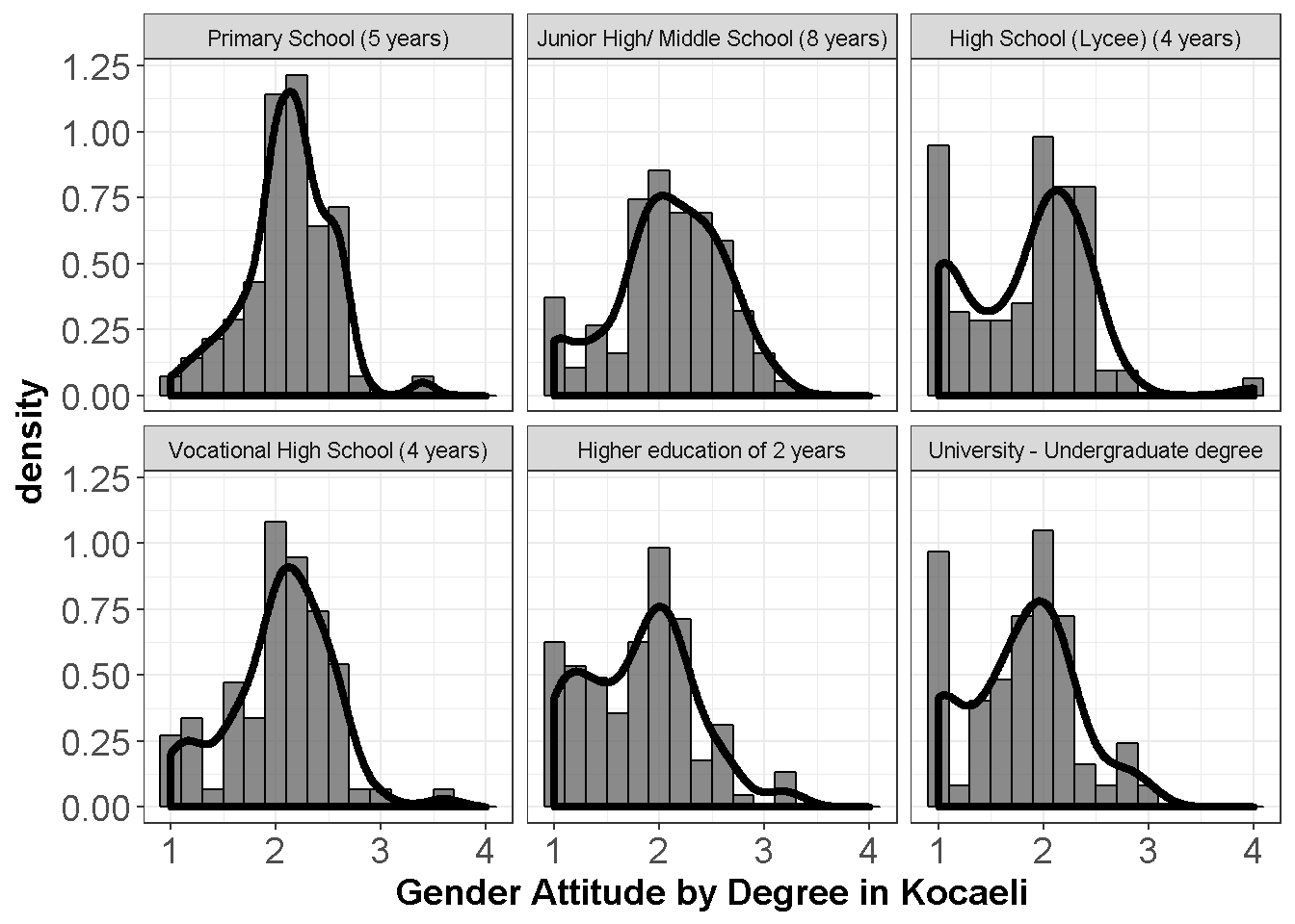
Figure 9.1: Gender Attitudes by Degree
Departures from the normality do not seem to be severe.
require(ggplot2)
ggplot(dataWBT_KOCAELI, aes(eduNEW,gen_att)) +
  geom_boxplot() +
  labs(x = "Education",y="Gender Attitude by degree in Kocaeli")+coord_flip()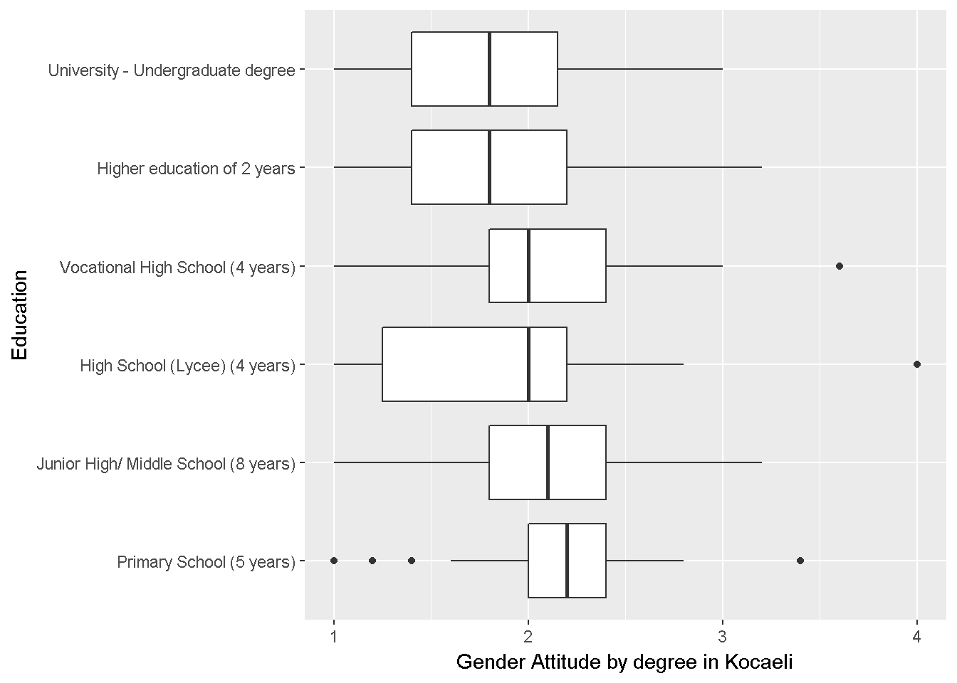
Figure 9.2: Gender Attitudes by Degree
Homogeneity of variance is questionable but not severely violated.
Step 3: Run ANOVA
For illustrative purposes, let us ignore the violations first. The ezANOVA function (Lawrence (2016)) reports the F test, the Levene Test and an effect size. Type of the effect size depends on the model. For further details, please carefully study the Table 1 in Bakeman (2005), an open access article, or Olejnik and Algina (2003). The Levene test rejects the null hypothesis of equal variances across factor levels.
library(ez)
#the ezANOVA function throws a warning if id is not a factor

dataWBT_KOCAELI$id=as.factor(dataWBT_KOCAELI$id)

# set the number of decimals (cosmetic)
options(digits = 3)


#alternative 1 the ezANOVA function

alternative1 = ezANOVA(
    data = dataWBT_KOCAELI,
    wid=id, dv = gen_att, between = eduNEW,observed=eduNEW)
## Warning: Data is unbalanced (unequal N per group). Make sure you specified
## a well-considered value for the type argument to ezANOVA().

alternative1
## $ANOVA
##   Effect DFn DFd    F        p p<.05    ges
## 1 eduNEW   5 564 7.27 1.31e-06     * 0.0605
##
## $`Levene's Test for Homogeneity of Variance`
##   DFn DFd  SSn  SSd   F      p p<.05
## 1   5 564 1.35 63.5 2.4 0.0361     *


# critical F value
qf(.95,5,564)
## [1] 2.23
ABOUT the warning of ez function;
#Warning: Data is unbalanced (unequal N per group). Make sure you specified
#a well-considered value for the type argument to ezANOVA().

ezANOVA can calculate three different types of sums of squares
for main effects and interactions.
For a one-way between-subjects design the F test is the same
for all three types and this warning can be ignored.
The same results can be obtained with the lm (linear model) function in R Core Team (2016b).
# alternative 2 the lm function
alternative2=lm(gen_att~eduNEW,data=dataWBT_KOCAELI)

#Table 2
anova(alternative2)
## Analysis of Variance Table
##
## Response: gen_att
##            Df Sum Sq Mean Sq F value    Pr(>F)
## eduNEW      5  10.13 2.02610  7.2676 1.306e-06 ***
## Residuals 564 157.24 0.27879
## ---
## Signif. codes:  0 '***' 0.001 '**' 0.01 '*' 0.05 '.' 0.1 ' ' 1
The aov function in R Core Team (2016b) is the third alternative.
#alternative 3 the aov function
alternative3=aov(gen_att~eduNEW,data=dataWBT_KOCAELI)
summary(alternative3)
##              Df Sum Sq Mean Sq F value   Pr(>F)
## eduNEW        5  10.13  2.0261   7.268 1.31e-06 ***
## Residuals   564 157.24  0.2788
## ---
## Signif. codes:  0 '***' 0.001 '**' 0.01 '*' 0.05 '.' 0.1 ' ' 1
The pairwise.t.test function in the stats package (R Core Team (2016b)) is convenient. Provide the preferred procedure by using p.adjust.method argument, for example p.adjust.method =“Holm” to use the adjustment given by Holm (1979). Five other procedures are available with this function, please see ?p.adjust.
# pairwise comparisons
# Table 3
with(dataWBT_KOCAELI, pairwise.t.test(gen_att,eduNEW,p.adjust.method ="holm"))
##
##  Pairwise comparisons using t tests with pooled SD
##
## data:  gen_att and eduNEW
##
##                                      Primary School (5 years)
## Junior High/ Middle School (8 years) 1.0000
## High School (Lycee) (4 years)        0.0040
## Vocational High School (4 years)     1.0000
## Higher education of 2 years          0.0014
## University - Undergraduate degree    0.0043
##                                      Junior High/ Middle School (8 years)
## Junior High/ Middle School (8 years) -
## High School (Lycee) (4 years)        0.0046
## Vocational High School (4 years)     1.0000
## Higher education of 2 years          0.0017
## University - Undergraduate degree    0.0057
##                                      High School (Lycee) (4 years)
## Junior High/ Middle School (8 years) -
## High School (Lycee) (4 years)        -
## Vocational High School (4 years)     0.0435
## Higher education of 2 years          1.0000
## University - Undergraduate degree    1.0000
##                                      Vocational High School (4 years)
## Junior High/ Middle School (8 years) -
## High School (Lycee) (4 years)        -
## Vocational High School (4 years)     -
## Higher education of 2 years          0.0176
## University - Undergraduate degree    0.0357
##                                      Higher education of 2 years
## Junior High/ Middle School (8 years) -
## High School (Lycee) (4 years)        -
## Vocational High School (4 years)     -
## Higher education of 2 years          -
## University - Undergraduate degree    1.0000
##
## P value adjustment method: holm
9.2.1.6 Robust estimation and hypothesis testing for a one-way between-subjects design
Several approaches to conducting a robust one-way between subjects ANOVA, have been presented by Wilcox (2012) One of the convenient robust procedure , a heteroscedastic one-way ANOVA for trimmed means, has been compressed into the t1way function, available via WRS-2 (Mair and Wilcox (2016)). Please use ?t1way for the current details, this promising package is being improved frequently .
library(WRS2)

#t1way
# 20% trimmed
t1way(gen_att~eduNEW,data=dataWBT_KOCAELI,tr=.2,nboot=5000)
## Call:
## t1way(formula = gen_att ~ eduNEW, data = dataWBT_KOCAELI, tr = 0.2,
##     nboot = 5000)
##
## Test statistic: 7.5658
## Degrees of Freedom 1: 5
## Degrees of Freedom 2: 143.78
## p-value: 0
##
## Explanatory measure of effect size: 0.29

# 10% trimmed
t1way(gen_att~eduNEW,data=dataWBT_KOCAELI,tr=.1,nboot=5000)
## Call:
## t1way(formula = gen_att ~ eduNEW, data = dataWBT_KOCAELI, tr = 0.1,
##     nboot = 5000)
##
## Test statistic: 9.5355
## Degrees of Freedom 1: 5
## Degrees of Freedom 2: 187.52
## p-value: 0
##
## Explanatory measure of effect size: 0.3

# 5% trimmed
t1way(gen_att~eduNEW,data=dataWBT_KOCAELI,tr=.05,nboot=5000)
## Call:
## t1way(formula = gen_att ~ eduNEW, data = dataWBT_KOCAELI, tr = 0.05,
##     nboot = 5000)
##
## Test statistic: 9.415
## Degrees of Freedom 1: 5
## Degrees of Freedom 2: 211.55
## p-value: 0
##
## Explanatory measure of effect size: 0.31

## heteroscedastic pairwise comparisons

#level order
lincon(gen_att~eduNEW,data=dataWBT_KOCAELI,tr=.1)[[2]]
## [1] "Higher education of 2 years"
## [2] "Junior High/ Middle School (8 years)"
## [3] "University - Undergraduate degree"
## [4] "Vocational High School (4 years)"
## [5] "High School (Lycee) (4 years)"
## [6] "Primary School (5 years)"
round(lincon(gen_att~eduNEW,data=dataWBT_KOCAELI,tr=.1)[[1]][,c(1,2,6)],3)
##       Group Group p.value
##  [1,]     1     2   0.701
##  [2,]     1     3   0.000
##  [3,]     1     4   0.360
##  [4,]     1     5   0.000
##  [5,]     1     6   0.000
##  [6,]     2     3   0.000
##  [7,]     2     4   0.597
##  [8,]     2     5   0.000
##  [9,]     2     6   0.000
## [10,]     3     4   0.004
## [11,]     3     5   0.460
## [12,]     3     6   0.467
## [13,]     4     5   0.001
## [14,]     4     6   0.003
## [15,]     5     6   0.911
9.2.1.7 Example write-up for one-way between-subjects ANOVA
For our illustrative example, results of hypothesis tests conducted using robust procedures did not disagree with the results of the ANOVA and pairwise comparisons of means. This was expected given the assumptions were not severely violated. When the robust analyses and conventional analyses yield the same decisions about all hypothesis tests, results of the conventional analyses can be reported due to their greater familiarity to most readers. A possible write up for our illustrative example would be:
An ANOVA was performed to investigate whether the gender attitudes scores differ across education level. The means,standard deviations, skewness and kurtosis values of the gender scores, grouped by the highest-degree obtained, are presented in Table 1. The analysis of variance indicated a significant difference in the gender attitudes scores , F(5,564) = 7.27, p < .001, \(\hat\eta^2_G=.06\). Table 2 is the ANOVA table for this analysis. Pairwise comparisons were planned a’ priori. The familywise error rate was selected for control and the Holm procedure (Holm (1979)) was used. The results of the pairwise comparisons are presented in Table 3. Nine out of fifteen comparisons yielded statistically significant results; (primary school vs lycee, primary school vs 2-year-collage, primary school vs undergraduate,… (provide details). Robust statistical procedures yielded the same conclusions.
9.2.1.8 Missing data techniques for one-way between-subjects ANOVA
To be added
9.2.1.9 Power calculations for one-way between-subjects ANOVA
To be added
9.2.2 Two-Factor Between Subjects ANOVA
This topic concerns designs in which there are two between-subjects factors: factor A with J levels and factor B with K levels for a total of JK combinations of levels; each combination is called a cell. The factors are between-subjects if (a) different subjects appear in each cell and (b) subjects are not matched in any way. In the simplest version of this design, each factor has two levels. For example, consider if a researcher is interested in the effect of the gender and college education on the gender attitudes scores. The following is a depiction of a study designed to investigate these two factors.
| non-college | college | ||
|---|---|---|---|
| Female | \(\mu_{11}\) | \(\mu_{12}\) | \(\mu_{1\cdot}\) |
| Male | \(\mu_{21}\) | \(\mu_{22}\) | \(\mu_{2\cdot}\) |
| \(\mu_{\cdot 1}\) | \(\mu_{\cdot 2}\) |
Also shown are the parameters about which hypotheses will be tested: the population cell means (\(\mu_{11}, \mu_{12}, \mu_{21},\mu_{22}\)), row means ( \(\mu_{1 \cdot}\), \(\mu_{2 \cdot}\)) and column means (\(\mu_{\cdot 1}\), \(\mu_{\cdot 2}\)). The general term for a row or column mean is a marginal mean.
Symbolically, the hypothesis of no interaction can be written as \(H_0: \mu_{11} - \mu_{12} = \mu_{21} - \mu_{22}\). The interation is also a comparison of the two simple effects of gender \((\mu_{21}−\mu_{11} and \mu_{22} − \mu_{12})\) leading to the null hypothesis \(H_0: \mu_{21}−\mu_{11}= \mu_{22}- \mu_{12}\). If one of the null hypotheses is true the other must also be true and if one is false the other must also be false.
Interaction The first null hypothesis of interest is the hypothesis of no interaction between the two factors. Before defining an interaction, we first define a simple main effect. A simple main effect refers to differences among the cell means in a particular row or in a particular column. In the current example, there are two types of simple main effects: simple main effects of gender and simple main effects of college education.
For each type, there are two simple main effects. There is a simple main effect of gender at college graduates (\(\mu_{12}\) versus \(\mu_{22}\)) and a simple main effect of gender at non-college graduates (\(\mu_{11}\) versus \(\mu_{21}\)).
There is a simple main effect of education for Female (\(\mu_{11}\) versus \(\mu_{12}\)) and a simple main effect of education for Male (\(\mu_{21}\) versus \(\mu_{22}\)).
The main effects Effects defined in terms of marginal (row and column) means are called main effects. Symbolically, the main effect of gender is \(\mu_{1\cdot} - \mu_{2\cdot}\), and the hypothesis of no main effect due to gender is \(H_0:\mu_{1\cdot} - \mu_{2\cdot} = 0\). Similarly, the hypothesis of no main effect due to college education is \(H_0:\mu_{\cdot 1} - \mu_{\cdot 2} = 0\).
When there is an interaction:
Inspection of the main effect for a factor is misleading when the directions of the simple main effects of the factor are not the same at all levels of the second factor.
It is a matter of opinion as to whether it is misleading to inspect the main effect for a factor the directions of the simple main effects of the factor are the same at all levels of the second factor.
When the main effect is misleading about the effect of a factor, the cell means are the proper basis for studying the effects of the factor.
The structural model for a two-factor between subjects ANOVA is \(Y_{ijk}=\mu+\alpha_{j}+\beta_k + \alpha\beta_{jk}+ \epsilon_{ij}\), in which \(Y_{ijk}\) is the score for the participant i in first factor level j , and the second factor level k; \(\mu\) is the grand mean of the scores, \(\alpha_j\) is the effect of the level j of the first factor, \(\beta_k\) is the effect of the level k of the second factor, \(\alpha\beta_{jk}\) is the interaction effect and \(\epsilon_{ij}\) is the error term (nuisance).
| SV | df | F |
|---|---|---|
| A | \(J-1\) | \(\frac{MS_A}{MS_{S/AB}}\) |
| B | \(K-1\) | \(\frac{MS_B}{MS_{S/AB}}\) |
| AB | \((J-1)(K-1)\) | \(\frac{MS_{AB}}{MS_{S/AB}}\) |
| S/AB | \(N-JK\) | |
| Total | \(N-1\) |
9.2.2.1 Type I, II and III sum of squares
As we pointed out in the section on one-way between-subjects designs, the F test of the main effect is the same for all three types of sums of squares. This is not true in designs with two or more between-subjects factors. In designs with three or more between-subjects of effects F tests for interaction other than the highest order interaction can vary across the types of sums of squares. Selecting among the three types can be an important decision and we refer the reader to Carlson and Timm (1974) for a discussion of the issues in selecting among the three types of sums of squares in experimental studies and to Appelbaum and Cramer (1976) for a discussion of the issues in survey studies.
9.2.2.2 R codes for a two-way between-subjects ANOVA
For illustrative purposes, the city of Kayseri is subsetted from the DataWBT (Section 2.3). The gender attitudes scores are the dependent variable, gender and higher education indicator are the between subjects factors.
Step 1: Set up data and report descriptive
# load csv from an online repository
urlfile='https://raw.githubusercontent.com/burakaydin/materyaller/gh-pages/ARPASS/dataWBT.csv'
dataWBT=read.csv(urlfile)

#remove URL
rm(urlfile)

#select the city of KAYSERI
# listwise deletion for gen_att and education variables
dataWBT_Kayseri=na.omit(dataWBT[dataWBT$city=="KAYSERI",c("id","gen_att","higher_ed","gender")])

# Higher education is coded as 0 and 1, change it to non-college, college
dataWBT_Kayseri$HEF=droplevels(factor(dataWBT_Kayseri$higher_ed,
                    levels = c(0,1),
                    labels = c("non-college", "college")))

#table(dataWBT_Kayseri$gender)
#table(dataWBT_Kayseri$HEF)

#drop empty levels
dataWBT_Kayseri$gender=droplevels(dataWBT_Kayseri$gender)

with(dataWBT_Kayseri,
     table(gender,HEF))
##         HEF
## gender   non-college college
##   Female          99      50
##   Male            67      36


# set the number of decimals (cosmetic)
options(digits = 3)

#get descriptives
library(doBy)
library(moments)
desc2BW=as.matrix(summaryBy(gen_att~HEF+gender, data = dataWBT_Kayseri,
          FUN = function(x) { c(n = sum(!is.na(x)),
                                mean = mean(x,na.rm=T), sdv = sd(x,na.rm=T),
                               skw=moments::skewness(x,na.rm=T),
                               krt=moments::kurtosis(x,na.rm=T)) } ))
# Table 4
desc2BW
##   HEF           gender   gen_att.n gen_att.mean gen_att.sdv gen_att.skw
## 1 "non-college" "Female" "99"      "1.93"       "0.424"     "-0.548"
## 2 "non-college" "Male"   "67"      "2.32"       "0.419"     "-0.191"
## 3 "college"     "Female" "50"      "1.80"       "0.346"     " 0.263"
## 4 "college"     "Male"   "36"      "2.13"       "0.543"     " 0.159"
##   gen_att.krt
## 1 "2.51"
## 2 "3.18"
## 3 "1.94"
## 4 "2.25"
#write.csv(desc2BW,file="twowayB_ANOVA_desc.csv")
Step 2: Inspect assumptions
require(ggplot2)
ggplot(dataWBT_Kayseri, aes(x = gen_att)) +
  geom_histogram(aes(y = ..density..),col="black",binwidth = 0.2,alpha=0.7) +
  geom_density(size=1.5) +
  theme_bw()+labs(x = "Gender Attitudes by HEF and Gender in Kayseri")+ facet_wrap(~ HEF+gender)+
  theme(axis.text=element_text(size=14),
        axis.title=element_text(size=14,face="bold"))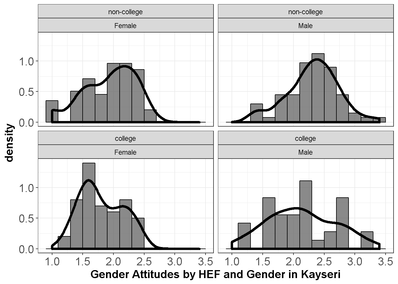
Figure 9.3: Gender Attitudes by HEF and Gender
Departures from the normality do not seem to be severe.
require(ggplot2)
ggplot(dataWBT_Kayseri, aes(x=gender, y=gen_att))+
  geom_boxplot()+
  facet_grid(.~HEF)+
  labs(x = "Gender",y="Gender Attitude by Gender and HEF in Kayseri")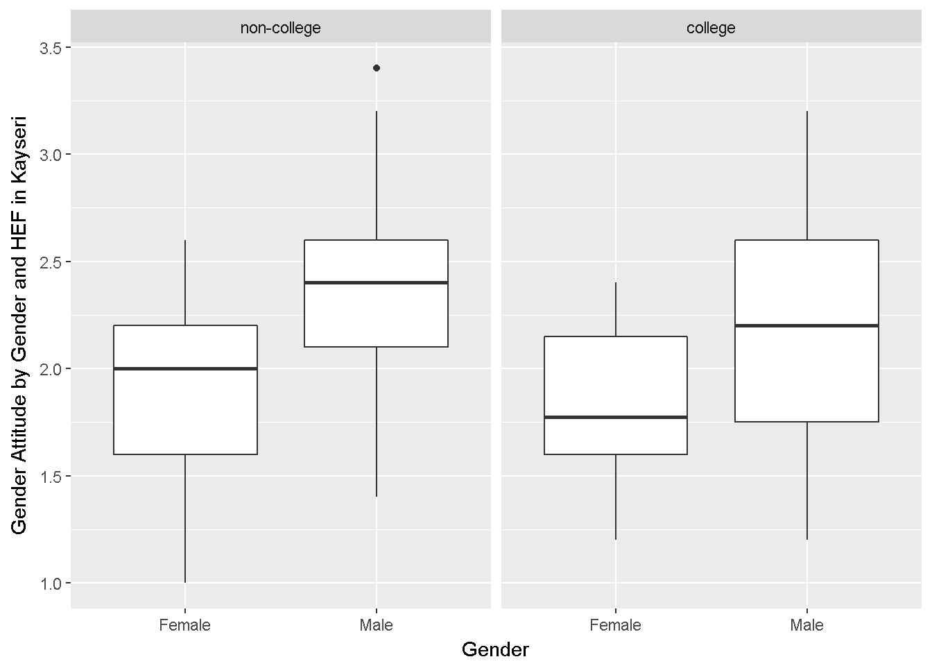
Figure 9.4: Gender Attitudes by Degree
Variances look similar.
Step 3: Run ANOVA
The ezANOVA function (Lawrence (2016)) reports the F test, the Levene Test and an effect size. Type of the effect size depends on the model and indirectly depends on the type of sum of squares used. The type argument (1,2 or 3) transmits the choice.
library(ez)
#the ezANOVA function throws a warning if id is not a factor

dataWBT_Kayseri$id=as.factor(dataWBT_Kayseri$id)

#alternative 1 the ezANOVA function
alternative1 = ezANOVA(
    data = dataWBT_Kayseri,
    wid=id, dv = gen_att, between = .(HEF,gender),observed=.(HEF,gender),type=2)
## Warning: Data is unbalanced (unequal N per group). Make sure you specified
## a well-considered value for the type argument to ezANOVA().

alternative1
## $ANOVA
##       Effect DFn DFd      F        p p<.05      ges
## 1        HEF   1 248  6.739 9.99e-03     * 0.022436
## 2     gender   1 248 45.389 1.12e-10     * 0.151106
## 3 HEF:gender   1 248  0.251 6.17e-01       0.000837
##
## $`Levene's Test for Homogeneity of Variance`
##   DFn DFd   SSn  SSd    F      p p<.05
## 1   3 248 0.469 17.5 2.22 0.0867


# Type III SS
# alternative1b = ezANOVA(
#     data = dataWBT_Kayseri,
#     wid=id, dv = gen_att, between = HEF+gender,type=3)
#
# alternative1b

# critical F value
qf(.95,1,248)
## [1] 3.88
9.2.2.3 Robust estimation and hypothesis testing for a two-way between-subjects design
Several approaches to conducting a robust two-way between subjects ANOVA, have been presented by Wilcox (2012) One of the convenient robust procedure , a heteroscedastic two-way ANOVA for trimmed means, has been compressed into the t2way function, available via WRS-2 (Mair and Wilcox (2016)). Please use ?t2way for the current details, this promising package is being improved frequently .
library(WRS2)

#t2way
# 20% trimmed
t2way(gen_att~HEF*gender,data=dataWBT_Kayseri,tr=.2)
## Call:
## t2way(formula = gen_att ~ HEF * gender, data = dataWBT_Kayseri,
##     tr = 0.2)
##
##              value p.value
## HEF         7.1310   0.011
## gender     20.2039   0.001
## HEF:gender  0.0855   0.772

# 10% trimmed
t2way(gen_att~HEF*gender,data=dataWBT_Kayseri,tr=.1)
## Call:
## t2way(formula = gen_att ~ HEF * gender, data = dataWBT_Kayseri,
##     tr = 0.1)
##
##              value p.value
## HEF         8.4235   0.005
## gender     33.1599   0.001
## HEF:gender  0.0361   0.850

# 5% trimmed
t2way(gen_att~HEF*gender,data=dataWBT_Kayseri,tr=.05)
## Call:
## t2way(formula = gen_att ~ HEF * gender, data = dataWBT_Kayseri,
##     tr = 0.05)
##
##              value p.value
## HEF         6.1688   0.015
## gender     29.8383   0.001
## HEF:gender  0.1642   0.687
9.2.2.4 Example write up two-way between-subjects ANOVA
For our illustrative example, robust procedures did not disagree with our initial analyses. This was expected given the assumptions were not severely violated. When the robust analyses yield very similar results, we prefer to report initial results to ease communication. A possible write up for our illustrative example would be:
Descriptive statistics for the gender attitudes scores as a function of gender and higher education in the city of Kayseri are presented in Table 4. A 2x2 ANOVA was reported. F tests were conducted at \(\alpha=.05\). There was a significant difference for gender \(F(1,248)=45.39, p<.001\). There was also a significant difference for the college effect \(F(1,248)=6.24, p=.013\). However, there was no significant interaction between the gender and higher education status, \(F(1,248)=0.25, p=.617\). The ezANOVA (Lawrence (2016)) function reported generalized eta hat squared (\(\hat\eta^2_G\)) of 0.15 for the gender effect and 0.02 for the college-effect. Table 5 is the ANOVA table for these analyses.
9.2.2.5 Follow ups for two-way between-subjects ANOVA
To be added.
9.2.2.5.1 Pairwise comparisons following two-way between-subjects ANOVA
To be added.
9.2.2.5.2 Contrats comparisons following two-way between-subjects ANOVA
To be added.
9.2.2.6 Missing data techniques for two-way between-subjects ANOVA
To be added
9.2.2.7 Power calculations for two-way between-subjects ANOVA
To be added
9.3 Within Subjects ANOVA
This procedure can be used when there are score on the same participants under several treatments or at several time points and is then called repeated measures ANOVA. It can also be used in blocking designs and is then called randomized block ANOVA. Compared to between-subjects designs, this procedure is expected to eliminate influence of individual differences, in other words, to reduced variability, and thus, to reduce error. This development results in more power than independent-samples ANOVA with the same sample size. Of course there are issues other than power that must be considered in selecting a design. For example, if the goal is to compare reading achievement under three instructional methods, using a design in which each participant is exposed to the three methods will be problematic because the effect of exposure to one treatment will continue to influence reading ability during the other treatments.
9.3.1 One-way Within-Subjects ANOVA
The structural model following Myers et al. (2013) notation for a non-additive model;
\[\begin{equation} Y_{ij}=\mu + \eta_i + \alpha_j + (\eta \alpha)_{ij} + \epsilon_{ij} \tag{9.1} \end{equation}\]where i represents the individual, i=1,…,n; j represents the levels of the within-subjects factor (i.e, the repeated measurement or the treatment factor), j=1,…,P. Y is the score; \(\mu\) is the grand mean; \(\eta_i\) represents the difference between individual’s average score over the levels and the grand mean; \(\alpha_j\) represents the difference between the average score under level j of the within-subjects factor and the grand mean; \((\eta \alpha)_ij\) represents the interaction, and \(\epsilon_{ij}\) represent the error component. Because \((\eta \alpha)_ij\) and \(\epsilon_{ij}\) have the same subscripts, they are confounded.
Generally, the interest is on \(\alpha_j\). This interest leads to hypothesis testing:
\[H_0: \mu_1 = \mu_2 = \cdots = \mu_P\]
The alternative hypothesis states that at least one population mean is different. The ANOVA table for a one-way with-subjects ANOVA is;
| SV | df | F |
|---|---|---|
| Subjects (S) | \(n-1\) | |
| Waves (A) | \(P-1\) | \(\frac{MS_A}{MS_{SA}}\) |
| SA | \((n-1)(P-1)\) | |
| Total | \(nP-1\) |
Note on additivity The simplest explanation of additivity is the situation that would justify \((\eta \alpha)_ij = 0\) in Equation (9.1). This unrealistic restriction implies that the effect of levels of the within-subject factor waves is the same for all individuals.
Shown below in Table 9.1 are data for an experiment in which each person participates in four treatments defined by the amount of alcohol consumed. The dependent variable is a reaction time measure.
| id | noALC | twoOZ | fouroz | sixoz |
|---|---|---|---|---|
| 1 | 1 | 2 | 5 | 7 |
| 2 | 2 | 3 | 5 | 8 |
| 3 | 2 | 3 | 6 | 8 |
| 4 | 2 | 3 | 6 | 9 |
| 5 | 3 | 4 | 6 | 9 |
| 6 | 3 | 4 | 7 | 10 |
| 7 | 3 | 4 | 7 | 10 |
| 8 | 6 | 5 | 8 | 11 |
Treatment means, treatment standard deviations, and subject means are shown below. A subject mean is the average of the four scores for that subject.
# set the number of decimals (cosmetic)
options(digits = 2)

#participants mean
apply(owadata,1, mean)
## [1] 3.2 4.0 4.4 4.8 5.4 6.0 6.2 7.6

#treatment mean
apply(owadata[,-1],2, mean)
##  noALC  twoOZ fouroz  sixoz
##    2.8    3.5    6.2    9.0

#treatment sd
apply(owadata[,-1],2,sd)
##  noALC  twoOZ fouroz  sixoz
##   1.49   0.93   1.04   1.31
Because each participant has a score for each treatment, amount of alcohol is a within-subjects factor and it is possible to calculate a correlation for each pair of treatments. These correlations, which are presented in Table 9.2, indicate that reaction time is highly correlated for each pair of treatments. Recall that corresponding to each correlation there is a covariance;
\[Cov_{pp^`}=S_pS_{p^`}r_{pp^`}\]
where \(p\) and \(p'\) are two levels of the alcohol consumption factor. For example the correlation between the scores in the first two levels of the alcohol consumption factor is \(r_{02}=0.93\). And the corresponding covariance is \(Cov_{02}=1.5*0.9*0.93=1.26\)
| noALC | twoOZ | fouroz | sixoz | |
|---|---|---|---|---|
| noALC | 1.00 | 0.93 | 0.88 | 0.88 |
| twoOZ | 0.93 | 1.00 | 0.89 | 0.94 |
| fouroz | 0.88 | 0.89 | 1.00 | 0.95 |
| sixoz | 0.88 | 0.94 | 0.95 | 1.00 |
The alcohol consumption factor is a within-subjects factor. Consequently the F statistic for comparing the four treatment means should be appropriate for a design with a within-subjects factor. Let
P = the number of levels of the within-subjects factor, in the example P=4 ;
\(\bar C\) = the average covariance; in the example \(\bar C\) = 1.26.
The appropriate F statistic is
\[F_W=\frac{MS_A}{MS_{SA}}=\frac{MS_A}{MS_{S/A}- \bar C}\]
where \(MS_A\) and \(MS_{S/A}\) are calculated as they are for a between-subjects factor and the W emphasizes the F statistic is for a within-subjects factor. The critical value is \(F_{\alpha,P-1,(P-1)(n-1)}\) . The denominator mean square, \(MS_{SA}\) , is read mean square Subjects x A where A is the generic label for the treatment factor. Recall that the F statistic for a between-subjects factor is \(F_B=MS_A/MS_{S/A}\). Comparison of \(F_W\) and \(F_B\) shows that \(F_W\) incorporates the correlations between the pairs of treatments and \(F_B\) does not. (Recall that, in like fashion, the dependent samples t statistic incorporates the correlation whereas the independent samples t statistic does not.) As a result, when applied to a design with a within-subjects factor \(F_W \geq F_B\).Therefore, incorrectly using will usually result in a loss of power.
9.3.1.1 Assumptions of one-way within-subjects ANOVA
Sphericity is an assumption about the pattern of variances and covariances.If the data are spherical, the difference between each pair of repeated measures has the same variance for all pairs.
Example covariance matrix;
| \(Y_1\) | \(Y_2\) | \(Y_3\) | |
|---|---|---|---|
| \(Y_1\) | 10 | 7.5 | 10 |
| \(Y_2\) | 7.5 | 15 | 12.5 |
| \(Y_3\) | 10 | 12.5 | 20 |
Sphericity holds;
| \(Y_p-Y_{p'}\) | \(\sigma^2_p + \sigma^2_{p'} - 2\sigma_{pp'}\) |
|---|---|
| \(Y_1-Y_2\) | 10+15-2(7.5)=10 |
| \(Y_1-Y_3\) | 10+20-2(10)=10 |
| \(Y_2-Y_3\) | 15+20-2(12.5)=10 |
Box’s epsilon —measures how severely sphericity is violated.
\[\frac{1}{P-1}\leq \epsilon \leq 1\]
Estimates of \(\epsilon\) are Greenhouse-Geisser (\(\hat \epsilon\)) and Huynh-Feldt (\(\tilde{\epsilon}\))
\(\tilde{\epsilon}\) can be larger than 1.0; if it is \(\tilde{\epsilon}\) is set equal to 1.0.
Critical value assuming sphericity is \(F_{alpha,(P-1),(n-1)(P-1)}\).
Approximately correct critical value when sphericity is violated \(F_{alpha,\epsilon (P-1),\epsilon (n-1)(P-1)}\).
normality of errors in Equation (9.1), \(\epsilon_{ij}\) is assumed to be normally and independently distributed with a mean value of zero.
normality of \(\eta_i\) in Equation (9.1), \(\eta_{i}\) is assumed to be normally and independently distributed with a mean value of zero.
Together the assumptions listed immediately above imply that the repeated measures are drawn from a multivariate normal distribution.
9.3.1.1.1 The relationship between additivity and sphericity
Although assumptions can be stated in terms of \(\eta_{i}\) and \(\epsilon_{ij}\), a simpler approach is that the repeated measures are drawn from a multivariate normal distribution with covariance matrix that meets the sphericity assumption. If the data meet the sphericity assumption, the difference between each pair of repeated measures has the same variance for all pairs.
Assuming that the data are drawn from a multivariate normal distribution and within each level of the within-subjects factor the scores are independent, having equal variance and covariances (compound symmetry) is a sufficient condition for the F test on the within-subjects factor to be valid.
If additivity holds and the equal variance assumption holds then compound symmetry holds. But compund symmetry is a stricter assumption than the sphericity. Considering that sphericity is a necessary and sufficient requirement for the F test on the within-subjects factor to be valid (assuming that data are drawn from a multivariate normal distribution and scores are independent within each level of the within-subjects factor) checking for spericity is more important than checking for additivity. In addition because there are adjusted degrees of freedom procedures that adjust the F test on the within-subjects factor for violation of sphericity, it is not necessary to test for additivity.
9.3.1.2 R codes for a one-way within-subjects ANOVA
For illustrative purposes, a subsample from an original cluster randomized trial study (for details see Daunic et al. (2012)) was taken. The subsample included 1 control-classroom and 17 students. The variable of interest is the problem solving knowledge. Each wave was approximately one year apart. Higher scores mean higher knowledge.
Step 1: Set up data
#enter data
PSdata=data.frame(id=factor(1:17),
                    wave1=c(20,19,13,10,16,12,16,11,11,14,13,17,16,12,12,16,16),
                    wave2=c(28,27,18,17,29,18,26,21,15,26,28,23,29,18,26,21,22),
                    wave3=c(21,24,14,8,23,15,21,15,12,21,23,17,26,18,14,18,19))
Report descriptive
# set the number of decimals (cosmetic)
options(digits = 3)

##the long format will be needed
#head(PSdata)
library(tidyr)
data_long = gather(PSdata, wave, PrbSol, wave1:wave3, factor_key=TRUE)

#get descriptives
library(doBy)
library(moments)
desc1W=as.matrix(summaryBy(PrbSol~wave, data = data_long,
          FUN = function(x) { c(n = sum(!is.na(x)),
                                mean = mean(x,na.rm=T), sdv = sd(x,na.rm=T),
                                skw=moments::skewness(x,na.rm=T),
                                krt=moments::kurtosis(x,na.rm=T)) } ))
# Table 6
desc1W
##   wave    PrbSol.n PrbSol.mean PrbSol.sdv PrbSol.skw PrbSol.krt
## 1 "wave1" "17"     "14.4"      "2.91"     " 0.311"   "2.10"
## 2 "wave2" "17"     "23.1"      "4.67"     "-0.224"   "1.64"
## 3 "wave3" "17"     "18.2"      "4.77"     "-0.315"   "2.45"
#write.csv(desc1W,file="onewayW_ANOVA_desc.csv")
The covariance matrix might be helpful.
# check covariance  Table 7
cov(PSdata[,-1])
##       wave1 wave2 wave3
## wave1  8.49  8.85  9.87
## wave2  8.85 21.81 18.49
## wave3  9.87 18.49 22.78
Step 2: Check assumptions
ggplot(data_long, aes(x=wave, y=PrbSol))+
  geom_boxplot()+
  labs(x = "Wave",y="Problem Solving Knowledge scores")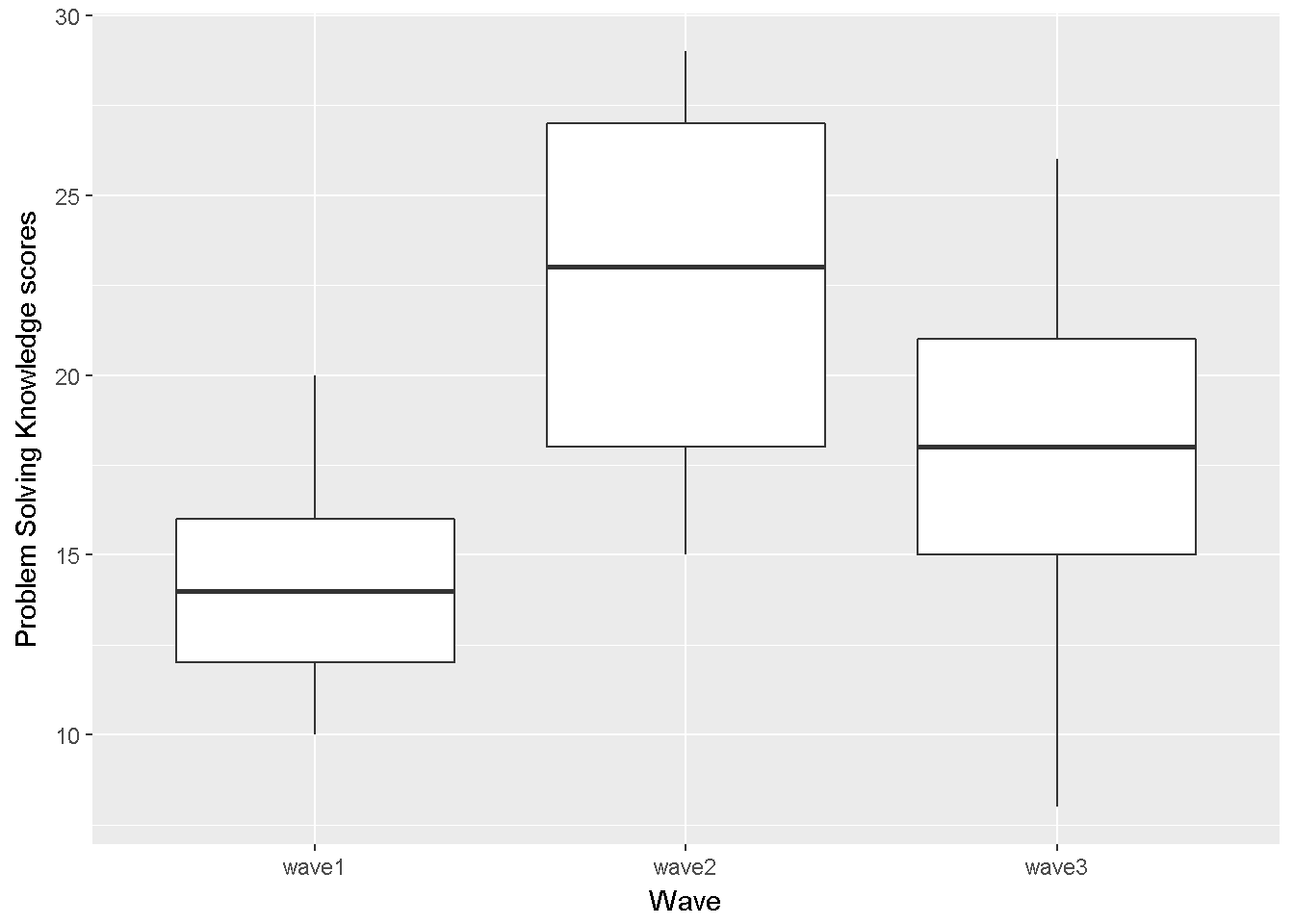
Figure 9.5: Problem Solving Knowledge score by wave
We will test for the sphericity assumption using Mauchly’s test integrated in the ezANOVA function, but this graph implies that it might be violated.
require(ggplot2)
ggplot(data_long, aes(x=wave, y=PrbSol, group=id))+
geom_line() + labs(x = "Wave",y="Problem Solving Knowledge scores")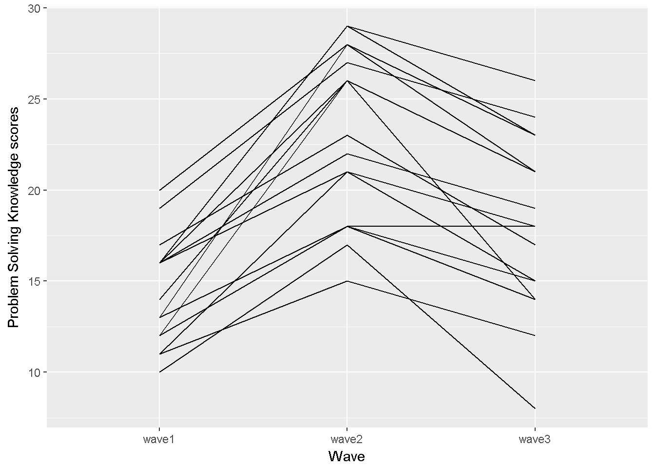
Figure 9.6: Problem Solving Knowledge score by wave, line graph
This graph, which plots the problem solving scores by wave, suggests that the \(\eta \beta_{ij}\) interaction terms are not likely to all be zero; therefore assuming sphericity while testing the hypothesis of equal wave means is not likely to be justified. The tukey.add.test function in asbio (Aho (2016)) investigates \(H_0\) : main effect and blocks are additive.
library(asbio)
with(data_long,tukey.add.test(PrbSol,wave,id))
##
## Tukey's one df test for additivity
## F = 5.943   Denom df = 31    p-value = 0.021

# if additivity exists a randomized block approach might be appropriate
#additive=with(data_long,lm(PrbSol~id+wave))
#anova(additive)
The Tukey additive test rejects the null hypothesis of additivity agrees with the line graph. In other words, a non-additive model is more appropriate for the problem solving knowledge data.
Step 3: Run ANOVA (including checks for the sphericity and normality of residuals assumptions)
The ezANOVA function (Lawrence (2016)) reports the F test, the Levene Test and an effect size. Type of the effect size depends on the model and indirectly depends on the type of sum of squares used, the type argument (1,2 or 3) transmits the choice.
library(ez)
#alternative 1 the ezANOVA function

alternative1 = ezANOVA(
    data = data_long,
    wid=id, dv = PrbSol, within = wave,
    detailed = T,return_aov=T)

alternative1
## $ANOVA
##        Effect DFn DFd   SSn SSd     F        p p<.05   ges
## 1 (Intercept)   1  16 17510 680 412.0 7.62e-13     * 0.954
## 2        wave   2  32   647 169  61.2 1.16e-11     * 0.433
##
## $`Mauchly's Test for Sphericity`
##   Effect     W     p p<.05
## 2   wave 0.918 0.526
##
## $`Sphericity Corrections`
##   Effect   GGe    p[GG] p[GG]<.05  HFe    p[HF] p[HF]<.05
## 2   wave 0.924 6.17e-11         * 1.04 1.16e-11         *
##
## $aov
##
## Call:
## aov(formula = formula(aov_formula), data = data)
##
## Grand Mean: 18.5
##
## Stratum 1: id
##
## Terms:
##                 Residuals
## Sum of Squares        680
## Deg. of Freedom        16
##
## Residual standard error: 6.52
##
## Stratum 2: id:wave
##
## Terms:
##                 wave Residuals
## Sum of Squares   647       169
## Deg. of Freedom    2        32
##
## Residual standard error: 2.3
## Estimated effects may be unbalancedPrbSolres=sort(alternative1$aov$id$residuals)
qqnorm(PrbSolres);qqline(PrbSolres)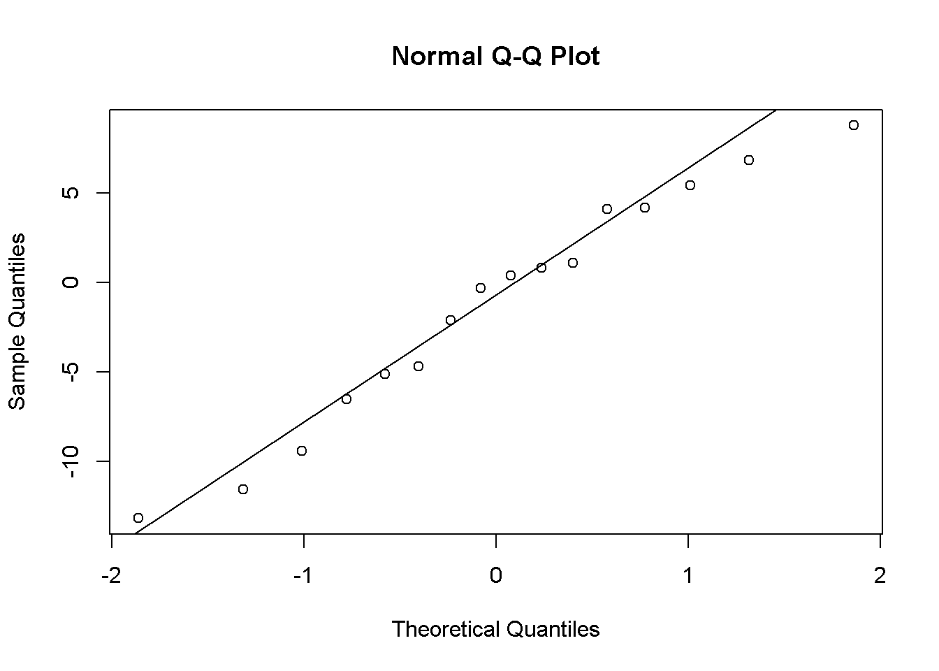
Figure 9.7: PSK model residuals
The distribution of the residuals is not severely non-normal.
The aov function is the second alternative.
# alternative 2 the aov function
summary(aov(PrbSol ~ wave + Error(id/wave), data=data_long))
##
## Error: id
##           Df Sum Sq Mean Sq F value Pr(>F)
## Residuals 16    680    42.5
##
## Error: id:wave
##           Df Sum Sq Mean Sq F value  Pr(>F)
## wave       2    647     324    61.2 1.2e-11 ***
## Residuals 32    169       5
## ---
## Signif. codes:  0 '***' 0.001 '**' 0.01 '*' 0.05 '.' 0.1 ' ' 1
9.3.1.3 Robust estimation and hypothesis testing for a one-way within-subjects design
One of the convenient robust procedures, a heteroscedastic one-way repeated measures ANOVA for trimmed means, has been compressed into the rmanova function, available via WRS-2 (Mair and Wilcox (2016)).
library(WRS2)

#rmanova
# 20% trimmed
with(data_long,rmanova(PrbSol,wave,id,tr=.20))
## Call:
## rmanova(y = PrbSol, groups = wave, blocks = id, tr = 0.2)
##
## Test statistic: 34.9
## Degrees of Freedom 1: 1.9
## Degrees of Freedom 2: 19
## p-value: 0
9.3.1.4 Example writeup one-way within-subjects ANOVA
Descriptive statistics for the problem solving knowledge scores at each wave are presented in Table 6. The covariance matrix is presented in Table 7. A one-way within ANOVA was reported. F test was conducted at \(\alpha=.05\). The assumptions of one-way within subjects ANOVA are satisfied. There was a significant difference between waves \(F(2,32)=61.2, p<.001\). The ezANOVA function reported a generalized eta hat squared (\(\hat\eta^2_G\)) of 0.43.
9.3.1.5 Follow ups for one-way within-subjects ANOVA
To be added.
9.3.1.6 Missing data techniques for one-way within-subjects ANOVA
To be added.
9.3.1.7 Power calculations for one-way within-subjects ANOVA
To be added.
9.4 Mixed Design
To be added.
References
Myers, Jerome L., A. Well, Robert F. Lorch, and Ebooks Corporation. 2013. Research Design and Statistical Analysis. 3rd ed. New York: Routledge.
Lawrence, Michael A. 2016. Ez: Easy Analysis and Visualization of Factorial Experiments. https://CRAN.R-project.org/package=ez.
Bakeman, Roger. 2005. “Recommended Effect Size Statistics for Repeated Measures Designs.” Behavior Research Methods 37 (3): 379–84. doi:10.3758/BF03192707.
Olejnik, Stephen, and James Algina. 2003. “Generalized Eta and Omega Squared Statistics: Measures of Effect Size for Some Common Research Designs.” Psychological Methods 8 (4): 434–47.
Wilcox, Rand R. 2012. Introduction to Robust Estimation and Hypothesis Testing. 3rd;3; US: Academic Press.
R Core Team. 2016b. R: A Language and Environment for Statistical Computing. Vienna, Austria: R Foundation for Statistical Computing. https://www.R-project.org/.
Holm, Sture. 1979. “A Simple Sequentially Rejective Multiple Test Procedure.” Scandinavian Journal of Statistics 6 (2): 65–70.
Mair, Patrick, and Rand Wilcox. 2016. WRS2: A Collection of Robust Statistical Methods. https://CRAN.R-project.org/package=WRS2.
Carlson, James E., and Neil H. Timm. 1974. “Analysis of Nonorthogonal Fixed-Effects Designs.” Psychological Bulletin 81 (9): 563–70.
Appelbaum, Mark I., and Elliot M. Cramer. 1976. “Balancing - Analysis of Variance by Another Name.” Journal of Educational Statistics 1 (3): 233–52.
Daunic, Ann P., Stephen W. Smith, Cynthia W. Garvan, Brian R. Barber, Mallory K. Becker, Christine D. Peters, Gregory G. Taylor, Christopher L. Van Loan, Wei Li, and Arlene H. Naranjo. 2012. “Reducing Developmental Risk for Emotional/Behavioral Problems: A Randomized Controlled Trial Examining the Tools for Getting Along Curriculum.” Journal of School Psychology 50 (2): 149–66.
Aho, Ken. 2016. Asbio: A Collection of Statistical Tools for Biologists. https://CRAN.R-project.org/package=asbio.
Removing this participant from the ANOVA would have had no substantial effect on the results.↩