8 Comparing Two Means, the t-test
Section 7.3.1 introduced the basics of a sampling distribution using the sample mean. When the interest is to compare two means the t-test is useful and the sampling distribution of the mean difference between two groups drives the analyses.
The mean of the sampling distribution of \(\bar{Y_1}-\bar{Y_2}\) \((\mu_{\bar{Y_1}-\bar{Y_2}})\) is always equal to \(\mu_1 - \mu_2\), but the standard deviation of the sampling distribution \((\sigma_{\bar{Y_1}-\bar{Y_2}})\) depends on the design used to collect the data.
Example: Consider an example in which the tensile strength of wounds closed by Suture and Tape is compared. The design for conducting this study will have one factor, Method of Wound Closure, with two levels, Tape and Suture. The following are two designs for conducting the study:
Within-subjects design. Incisions are made on both sides of the spine for each of 10 rats. Tape was used to close one of the wounds; the other was sutured. For each rat the wound closed by tape was determined randomly. This design is called within-subjects because the measurements under tape and suture are made on the same rat; rats are the subjects in the study.
Between-subjects design. Beginning with 20 rats, 10 are randomly assigned to have a wound closed by tape and the other 10 rats have a wound closed by suture. For each rat an incision is made on one side of the spine. The side is determined randomly for each rat.(Half of the rats assigned to each closure method have the incison on the left side of the spine and half on the right side. We ignore side of the spine as a factor in this example.) This design is called between-subjects because the measurements under tape and suture are made on different rats. An additional requirement for classifying the design as between-subjects is that no attempt was made to match the rats prior to random assignment. For example if the 20 rats were from 10 litters with different parents, the rats might have been matched on litter prior to random assignment.
One can imagine a population mean and a population standard deviation under each closure method.
For example the population mean under tape closure is the mean for an indefinitely large group of rats all of which have a wound closed by tape.
In the following comparison it is assumed that the population mean for tape closing will be the same in the within-subjects and the between-subjects design and that the population standard deviation will be the same in the within-subjects and the between-subjects design.
The corresponding assumptions for the population mean and standard deviation for the suture closing are made.
The following are the symbols for these population parameters.
| Parameter for Population | Tape | Suture |
|---|---|---|
| Mean | \(\mu_T\) | \(\mu_S\) |
| Standard deviation | \(\sigma_T\) | \(\sigma_S\) |
| Sample size | \(n_T\) | \(n_S\) |
Note. More generally, \(\mu_1\) and \(\mu_2\) for population means for the two treatments and \(\sigma_1\) and \(\sigma_2\) for population standard deviations for the two treatments.
| Parameter for Sampling Distribution | Between-Subjects | Within-Subjects |
|---|---|---|
| Mean (\(\mu_{\bar{Y_T}-\bar{Y_S}}\)) | \(\mu_T-\mu_S\) | \(\mu_T-\mu_S\) |
| Standard deviation (\(\sigma_{\bar{Y_T}-\bar{Y_S}}\)) | \(\sqrt{\frac{\sigma_T^2+\sigma_S^2}{n}}\) | \(\sqrt{\frac{\sigma_T^2+\sigma_S^2-2\sigma_T \sigma_S \rho_{TS}}{n}}\) |
\(\rho_{TS}\) is the correlation between the tensile strength scores in the tape and suture treatments in the within-subjects design.
The difference in the standard errors is due to \(\rho_{TS}\). If this correlation is zero the designs result in the same standard error.
An important goal in designing a study is to make the standard error as small as possible. When the standard error is small the statistic in which we are interested will tend to be close in numeric value to the parameter we are estimating.
In data analysis we must select a formula for a standard error (or for the error variance). Selecting the wrong formula is a critical error in data analysis.
In practice the standard error is selected by classifying the design as between-subjects or within subjects. This means that incorrectly classifying the design is a critical error in data analysis.
8.1 Between-Subjects t-test (The Independent Groups t-test)
The gender attitudes scores for college graduates vs non-collage graduates in the city of USAK are compared. The density plot for each group’s gender attitudes scores is shown below.
# load csv from an online repository
urlfile='https://raw.githubusercontent.com/burakaydin/materyaller/gh-pages/ARPASS/dataWBT.csv'
dataWBT=read.csv(urlfile)

#remove URL
rm(urlfile)
dataWBT_USAK=dataWBT[dataWBT$city=="USAK",]


# We explained the functions 'factor' and 'droplevels' in section 5.2.4
# here we create a factor, Higher Education Factor (HEF).
# it is labeled as 'non-college' when the higher_ed variable equals 0,
# 'college' when equals to 1.
# if you dont use droplevels function, you might have an empty level
dataWBT_USAK$HEF=droplevels(factor(dataWBT_USAK$higher_ed,
                    levels = c(0,1),
                    labels = c("non-college", "college")))

require(ggplot2)
plotdata=na.omit(dataWBT_USAK[,c("gen_att","HEF")])
ggplot(plotdata, aes(x = gen_att)) +
  geom_histogram(aes(y = ..density..),col="black",binwidth = 0.2,alpha=0.7) +
  geom_density(size=2) +
  theme_bw()+labs(x = "Gender Attitude by HEF in USAK")+ facet_wrap(~ HEF)+
  theme(axis.text=element_text(size=15),
        axis.title=element_text(size=14,face="bold"))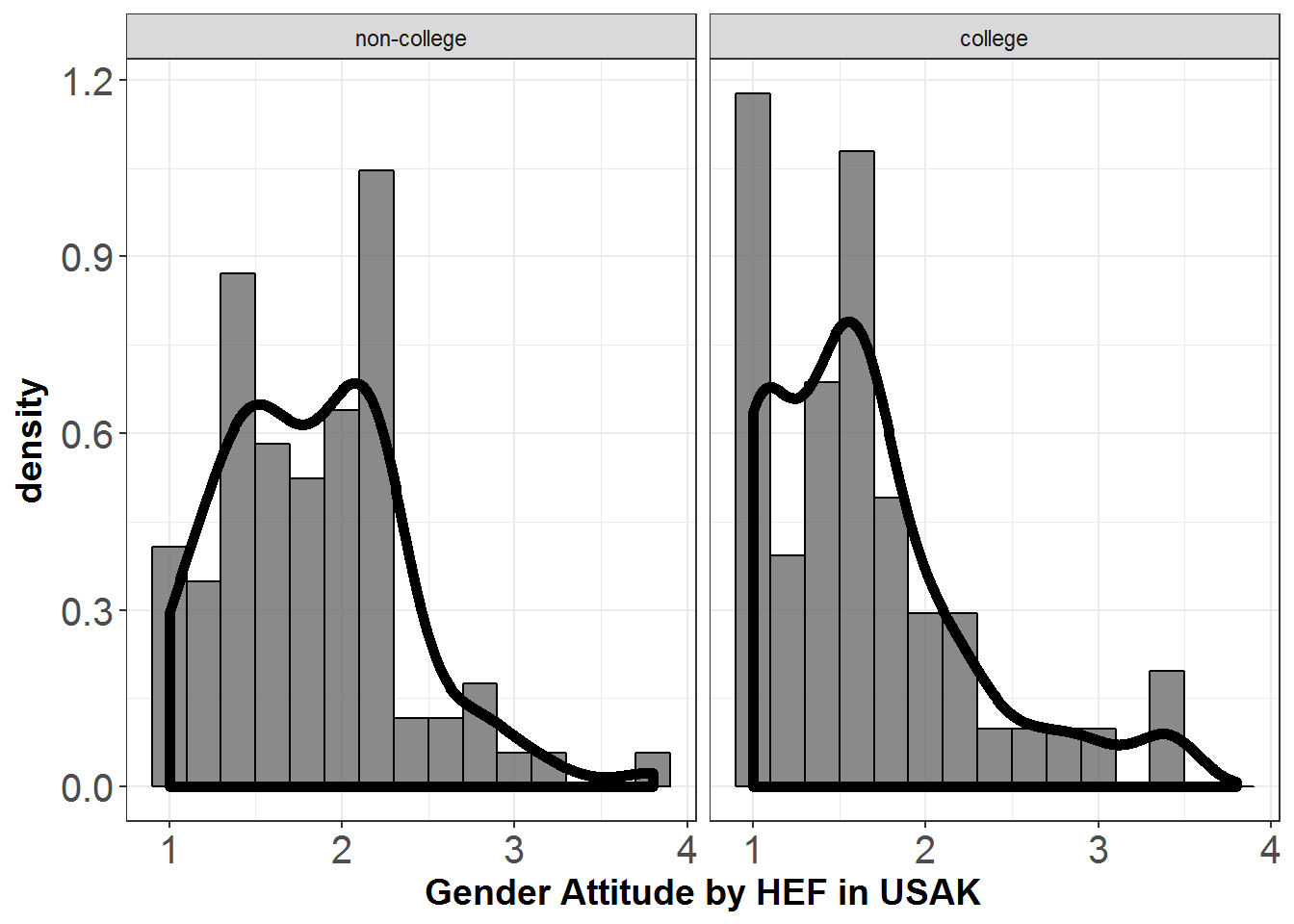
Figure 8.1: Gender Attitudes by Treatment Group
8.1.1 R codes for the independent groups t-test
The following are the steps for conducting the independent groups t-test and R code for implementing the steps
- Create descriptive statistics
- Calculate the test statistic
\[t=\frac{\bar{Y_1}-\bar{Y_2}}{S_p \sqrt{\frac{1}{n_1}+\frac{1}{n_2}}}\]
\[ S_p = \sqrt{\frac{(n_1-1)S_1^2 + (n_2-1)S_2^2 }{n_1+n_2-2}} \] 3. Find the critical value \(\pm t_{\alpha/2,n_1+n_2-2}\)to test \[H_0:\mu_1-\mu_2=0\] \[H_1:\mu_1-\mu_2 \neq0\]
library(psych)
descIDT=with(dataWBT_USAK,describeBy(gen_att, HEF,mat=T,digits = 2))
descIDT
##     item      group1 vars  n mean   sd median trimmed  mad min max range
## X11    1 non-college    1 86 1.83 0.54    1.8    1.80 0.59   1 3.8   2.8
## X12    2     college    1 51 1.64 0.61    1.6    1.54 0.59   1 3.4   2.4
##     skew kurtosis   se
## X11 0.72     0.90 0.06
## X12 1.19     1.09 0.09
#write.csv(descIDT,file="independent_t_test_desc.csv")

# Pooled sd
sp=sqrt((85*.543^2 + 50*.608^2)/(86+51-2))

# t-statistic
tstatistic=(1.832-1.635)/(sp*sqrt(1/86+1/51))

# critical value for alpha=0.05
qt(.975,df=135)
## [1] 1.977692
Since 1.963 is smaller than the critical value of \(t_{.975,135}=1.978\) , \(H_0\) is retained.
For \(H_1:\mu_1-\mu_2 > 0\), the critical value is \(t_{.95,135}=1.66\) which would yield the rejection of \(H_0\) given 1.93 is greater than 1.66.
For \(H_1:\mu_1-\mu_2 < 0\), the critical value is \(t_{.05,135}=-1.66\) which would yield the retaining of \(H_0\) given 1.93 is not lower than -1.66.
A more convenient R code would be;
# The dataWBT does not have HEF factor,
# you should define it as it is given a few lines above.

t.test(gen_att~HEF,data=dataWBT_USAK,var.equal=T,
                                     alternative="two.sided",
                                     conf.level=0.95)
##
##  Two Sample t-test
##
## data:  gen_att by HEF
## t = 1.9587, df = 135, p-value = 0.05221
## alternative hypothesis: true difference in means is not equal to 0
## 95 percent confidence interval:
##  -0.001903268  0.394880924
## sample estimates:
## mean in group non-college     mean in group college
##                  1.831783                  1.635294

# greater
t.test(gen_att~HEF,data=dataWBT_USAK,var.equal=T,
                                     alternative="greater",
                                     conf.level=0.95)
##
##  Two Sample t-test
##
## data:  gen_att by HEF
## t = 1.9587, df = 135, p-value = 0.0261
## alternative hypothesis: true difference in means is greater than 0
## 95 percent confidence interval:
##  0.03034529        Inf
## sample estimates:
## mean in group non-college     mean in group college
##                  1.831783                  1.635294


# less
t.test(gen_att~HEF,data=dataWBT_USAK,var.equal=T,
                                     alternative="less",
                                     conf.level=0.95)
##
##  Two Sample t-test
##
## data:  gen_att by HEF
## t = 1.9587, df = 135, p-value = 0.9739
## alternative hypothesis: true difference in means is less than 0
## 95 percent confidence interval:
##       -Inf 0.3626324
## sample estimates:
## mean in group non-college     mean in group college
##                  1.831783                  1.635294
8.1.1.1 Write up for non-directional test:
An independent groups t-test showed that in the city of USAK, the gender attitudes scores for the college graduates (n=51, mean=1.64, SD=0.61, skew=1.19, kurtosis=1.09) were not statistically different than the non-college graduates (n=86, mean=1.83, SD=0.54, skew=0.72, kurtosis=0.90), t(135)=1.96, p=0.052. The 95% confidence interval was [-0.002,0.395].10:
8.1.1.2 Write up for directional test:
A directional independent groups t-test showed that in the city of USAK, the gender attitudes scores for the college graduates (n=51, mean=1.64, SD=0.61, skew=1.19, kurtosis=1.09) were significantly lower than the non-college graduates (n=86, mean=1.83, SD=0.54, skew=0.72, kurtosis=0.90), t(135)=1.96, p=0.026. The 95% confidence interval was [0.030,\(\infty\)].
8.1.2 Assumptions of the independent groups t-test
Three assumptions should be met to claim statistical validity for a conventional between-subjects t-test.
Independence . The scores in each group should be independently distributed. The validity of this assumption is questionable when (a) scores for participants within a group are collected over time or (b) the participants within a group work together in a manner such that a participant’s response could have been influenced by another participant in the study. (See 9.2.1.4 for additional discussion)
Normality. The scores with each group are drawn from a normal distribution. However Myers et al. (2013) states that when the two groups are equal in size and the total sample size is 40 or larger departures from normality can be tolerated unless the scores are drawn from extremely skewed distributions. As noted earlier, the authors of the current book are hesitant to conduct tests for normality. However the use of robust procedures is advised when there is doubt for the normality.
Equal variance. This assumption is also called the homogeneity of variance assumption and means it is assumed that samples in the two groups are drawn from two populations with equal variances. Myers et al. (2013) states that when the sample sizes are equal and larger than 5, even with very large variance ratios (\(s_1^2/s_2^2=100\)) the conventional t-test leads to acceptable Type-I error rates. However this not the case with unequal sample sizes. Field, Miles, and Field (2012) states that tests for the variance homogeneity, i.e. Levene, might not perform well with small and unequal sample sizes. The problems with tests on variance are that they are not powerful enough to detect inequality of variance even when it is large enough to cause problems with the t test and most are less robust to non-normality than the t test is. The t.test function , by default, does not assume equal variances and uses a Welch’s t-test.
Even though we briefly summarized the assumptions of the independent groups t-test above, they were only introductory. For example we did not discuss violating equal variance and normality simultaneously. The discussion of what is “acceptable” is another limitation for our brief summary, for example when n1 = n2 = 10 we estimated the Type I error rate for \(\alpha = .01\) and a non-directional test to be .018 based on a 100000 replications. Most people would see .018 as liberal with \(\alpha = .01\)
There is an enormous literature on the effects of violating the assumptions of the independent samples t test on both Type I error rate and power and a great deal is known about when the independent samples t test works well and when it does not. However, because that literature is so large it is difficult to summarize it in a way that will allow data analysts to decide in every situation if the independent samples t test should be used. Perhaps a reasonable summary is that if independence appears to be violated an appropriate alternative to the independent sample t test should be used. If independence does not appear to be violated, then when the sample sizes are equal and at least 20 in each group and the scores are approximately normally distributed the independent samples t test can be used. In other situations alternatives to the independent samples t test should be used.
8.1.3 Using Welch’s t test
Welch’ t-test can be conveniently implemented in R and is a reasonable choice for comparing means for independent groups when the normality is not severely violated, the groups have different sample sizes and each groups’ sample size is reasonable large, (e.g. > 20) , and the homogeneity of variance assumption is not made.
t.test(gen_att~HEF,data=dataWBT_USAK,var.equal=F,
                                     alternative="two.sided",
                                     conf.level=0.95)
##
##  Welch Two Sample t-test
##
## data:  gen_att by HEF
## t = 1.9028, df = 95.885, p-value = 0.06006
## alternative hypothesis: true difference in means is not equal to 0
## 95 percent confidence interval:
##  -0.008484626  0.401462282
## sample estimates:
## mean in group non-college     mean in group college
##                  1.831783                  1.635294
8.1.3.1 Write up for non-directional Welch’s t-test:
An independent groups Welch’s t-test showed that in the city of USAK, the gender attitudes scores for the college graduates (n=51, mean=1.64, SD=0.61, skew=1.19, kurtosis=1.09) were not statistically different than the non-college graduates (n=86, mean=1.83, SD=0.54, skew=0.72, kurtosis=0.90), t(95.89)=1.90, p=0.06. The 95% confidence interval was [-0.008,0.402].
When the departures from the normality is severe, especially when the groups demonstrate substantially different distributions, a percentile bootstrap procedure is effective (Wilcox (2012),page 171).
#Calculate 95% CI using bootstrap (normality is not assumed)
set.seed(04012017)
B=5000       # number of bootstraps
alpha=0.05   # alpha

# define groups
GroupCollege=na.omit(dataWBT_USAK[dataWBT_USAK$HEF=="college","gen_att"])
GroupNONcollege=na.omit(dataWBT_USAK[dataWBT_USAK$HEF=="non-college","gen_att"])

output=c()
for (i in 1:B){

  x1=mean(sample(GroupCollege,replace=T,size=length(GroupCollege)))
  x2=mean(sample(GroupNONcollege,replace=T,size=length(GroupNONcollege)))
  output[i]=x2-x1
  }
output=sort(output)

## non-directional
# D star lower
output[as.integer(B*alpha/2)+1]
## [1] -0.01338349

# D star upper
output[B-as.integer(B*alpha/2)]
## [1] 0.3899111

##Directional x2>x1
# D star lower
output[as.integer(B*alpha)+1]
## [1] 0.02202462

#wrong direction x2<x1
# D star upper
output[as.integer(B*(1-alpha))]
## [1] 0.3575695
8.1.3.2 Write up for percentile bootstrap method:
In the city of USAK, the gender attitudes scores for the college graduates (n=51, mean=1.64, SD=0.61, skew=1.19, kurtosis=1.09) were not statistically different than the non-college graduates (n=86, mean=1.83, SD=0.54, skew=0.72, kurtosis=0.90) given that the 95% confidence interval was [-0.013,0.390].11
For a directional test: When the direction is appropriately stated in the alternative hypothesis, the lower limit of the 95% CI is 0.022 and yields the rejection of the null hypothesis of \(H_0:\mu_{non-college} = \mu_{college}\) in favor of \(H_1:\mu_{non-college}-\mu_{college} > 0\).
For a directional test: When the direction is NOT appropriately stated in the alternative hypothesis, the upper limit of the 95% CI is 0.358 and yields the retaining of the null hypothesis of \(H_0:\mu_{non-college} = \mu_{college}\) against the \(H_1:\mu_{non-college}-\mu_{college} < 0\).
8.1.4 Effect size for the independent groups t-test
A t statistic tells whether the mean difference is large in a statistical sense but not in a substantive sense. To judge whether a mean difference is large in a substantive sense one can use an effect size. Cohen’s effect size is the difference between the means divided by the pooled standard deviation and can be computed using; \[ES=\frac{t}{\sqrt{\frac{n_1n_2}{n_1+n_2}}}\]
Effect sizes are often judged in terms of criteria suggested by Cohen (1962).
| Effect Size | Description |
|---|---|
| .2 | Small |
| .5 | Medium |
| .8 | Large |
##  the normality and the equal variances assumptions are made
## given the robust procedures provided roughly the same results
n1=51
n2=86
tval=1.96

ES=tval/sqrt((n1*n2)/(n1+n2))
ES
## [1] 0.3464033

#or by the package effsize
t.test(gen_att~HEF,data=dataWBT_USAK,var.equal=F,
                                     alternative="two.sided",
                                     conf.level=0.95)
##
##  Welch Two Sample t-test
##
## data:  gen_att by HEF
## t = 1.9028, df = 95.885, p-value = 0.06006
## alternative hypothesis: true difference in means is not equal to 0
## 95 percent confidence interval:
##  -0.008484626  0.401462282
## sample estimates:
## mean in group non-college     mean in group college
##                  1.831783                  1.635294
library(effsize)
cohen.d(gen_att~HEF,data=dataWBT_USAK, paired=F, conf.level=0.95,noncentral=F)
##
## Cohen's d
##
## d estimate: 0.346177 (small)
## 95 percent confidence interval:
##          inf          sup
## -0.005791781  0.698145741
# experiment noncentral=T.
The effsize package (Torchiano 2016) reported an effect size of 0.35 with a 95% CI of [-0.008, 0.701]
8.1.5 Extra: Practical significance vs statistical significance
There are a number of points to keep in mind about practical significance (a term similar to practical significance is clinical significance.) versus statistical significance.
What do these terms mean? In treatment studies, statistically significant means large enough to be unlikely to have occurred by sampling error if the population means are equal whereas practically significant means large enough to be judged as practically important. Note then that significant has a different meaning in the two terms.
In treatment studies, practical significance can be measured by the mean difference or, when the scale of measurement is not well understood, by the effect size.
The claim is sometimes made that and effect can be practically significant but not statistically significant. This would mean that the effect is judged to be large but is not statistically significant. The problem with this claim is that an effect that is large but not statistically significant can only occur in a small study. Therefore the effect will be imprecisely estimated, which undermines the credibility of the claim that the effect is practically significant.
Another claim sometimes made is that an effect can be statistically significant, but not practically significant. This claim can be correct. For example, suppose there were 400 participants in an experiment, resulting in 200 participants in each group. The researcher found a small ES of 0.20 which is significantly different than zero (t = 2, p < .05). If we regard an effect size of .2 as not practically significant then we have an effect that is statistically, but not practically significant.
8.1.6 Missing data techniques for the independent groups t-test
To be added
8.1.7 Supportive graphs for the independent groups t-test
To be added
8.1.8 Power calculations for the independent groups t-test
Section 7.3.8 provided the basics of statistical power.
#power.t.test
power.t.test(delta=.35, sd=.6,sig.level=0.05, power=0.95,
             type="two.sample", alternative="two.sided")
##
##      Two-sample t test power calculation
##
##               n = 77.35093
##           delta = 0.35
##              sd = 0.6
##       sig.level = 0.05
##           power = 0.95
##     alternative = two.sided
##
## NOTE: n is number in *each* group
This illustration shows that for the pre-determined knowns of a mean difference of 0.35, a standard deviation of 0.6, an alpha level of 0.05, a non-directional test and a desired power of 0.95, the sample size should be 78 in each group. In other words, the probability of rejecting the null (\(H_0:\mu_1-\mu_2=0\)) is .95 with a sample size of 156, a mean difference of 0.35, SD=0.6, alpha=0.05 and a non-directional independent t-test.
8.2 The dependent groups t-test (Within-subjects t-test)
To examine whether surgical tape or suture is a better method for closing wounds, for each of 20 rats incisions were made on both sides of the spine. One of the wounds was closed by using tape; the other was sutured. The side closed by tape was determined at random. After 10 days the tensile strength of the wounds was measured. The following are the data.
wounds=data.frame(ratid=1:20,
                  tape=c(6.59,9.84 ,3.97,5.74,4.47,4.79,6.76,7.61,6.47,5.77,
                         7.36,10.45,4.98,5.85,5.65,5.88,7.77,8.84,7.68,6.89),
                  suture=c(4.52,5.87,4.60,7.87,3.51,2.77,2.34,5.16,5.77,5.13,
                           5.55,6.99,5.78,7.41,4.51,3.96,3.56,6.22,6.72,5.17))

# Create plot data
library(tidyr)
plotdata=gather(wounds, method, strength, tape:suture, factor_key=TRUE)

require(ggplot2)
ggplot(plotdata, aes(x = strength)) +
  geom_histogram(aes(y = ..density..),col="black",alpha=0.7) +
  geom_density(size=2) +
  theme_bw()+labs(x = "strength")+ facet_wrap(~ method)+
  theme(axis.text=element_text(size=15),
        axis.title=element_text(size=14,face="bold"))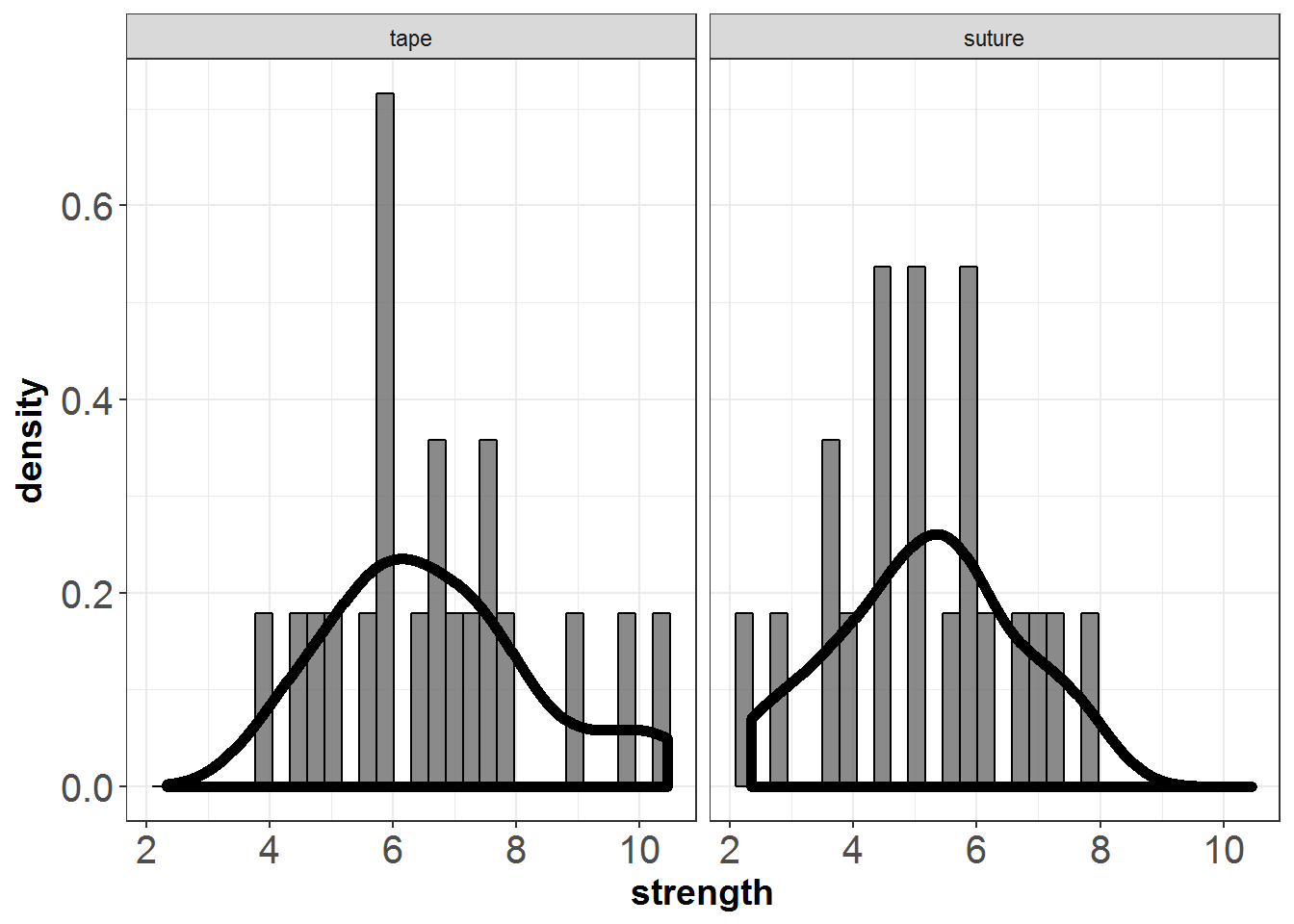
Figure 8.2: Wounds example
8.2.1 R codes for the dependent groups t-test
The following are the steps for conducting the dependent groups t-test and R code for implementing the steps
- Create descriptive statistics
- Calculate the test statistic
\[t=\frac{\bar{Y_1}-\bar{Y_2}}{\sqrt{\frac{S_1^2+S_2^2-2S_1 S_2 r_{12}}{n}}}\]
- Find the critical value \(\pm t_{\alpha/2,n-1}\)to test \[H_0:\mu_1-\mu_2=0\] \[H_1:\mu_1-\mu_2 \neq0\]
library(psych)
descDT=with(wounds,describe(cbind(tape,suture)))
descDT
##        vars  n mean   sd median trimmed  mad  min   max range  skew
## tape      1 20 6.67 1.71   6.53    6.54 1.45 3.97 10.45  6.48  0.55
## suture    2 20 5.17 1.49   5.17    5.19 1.30 2.34  7.87  5.53 -0.08
##        kurtosis   se
## tape      -0.45 0.38
## suture    -0.87 0.33

corDT=with(wounds,cor(tape,suture,use="complete.obs"))
corDT
## [1] 0.3536491


# estimated standard error
ese=sqrt(((1.71^2+1.49^2)-(2*1.71*1.49*corDT))/(20))

# t-statistic
tstatistic=(6.67-5.17)/ese

# critical value for alpha=0.05
qt(.975,df=19)
## [1] 2.093024
Given 3.67 is grater than the critical value of \(t_{.975,19}=2.09\) , \(H_0\) is rejected
A more convenient R code would be;
library(psych)
with(wounds, t.test(tape,suture,paired=T,
                                     alternative="two.sided",
                                     conf.level=0.95))
##
##  Paired t-test
##
## data:  tape and suture
## t = 3.6678, df = 19, p-value = 0.001636
## alternative hypothesis: true difference in means is not equal to 0
## 95 percent confidence interval:
##  0.6429426 2.3520574
## sample estimates:
## mean of the differences
##                  1.4975
8.2.1.1 Write up for non-directional dependent groups t-test:
A dependent groups t-test showed that the tensile strength after surgical tape (mean=6.67, SD=1.71, skew=0.55, kurtosis=-0.45) was statistically different than the tensile strength after the suture (mean=5.17, SD=1.49, skew=-0.08, kurtosis=-0.87), t(19)=3.67, p=0.002 ,r=0.35. The 95% confidence interval was [0.64,2.35].
8.2.2 Assumption for the dependent groups t-test
The score difference (\(Y_{1i} - Y_{2i}\)) should be normally distributed and the difference scores should be independent.However,the dependent t test is expected to be robust to normality with large sample sizes.
8.2.3 Robust estimation for the dependent groups t-test
When the departures from the normality is severe, a percentile bootstrap procedure can be employed (Wilcox (2012),page 201).
#Calculate 95% CI using bootstrap (normality is not assumed)
set.seed(04012017)
B=5000       # number of bootstraps
alpha=0.05   # alpha

wounds=data.frame(ratid=1:20,
                  tape=c(6.59,9.84 ,3.97,5.74,4.47,4.79,6.76,7.61,6.47,5.77,
                         7.36,10.45,4.98,5.85,5.65,5.88,7.77,8.84,7.68,6.89),
                  suture=c(4.52,5.87,4.60,7.87,3.51,2.77,2.34,5.16,5.77,5.13,
                           5.55,6.99,5.78,7.41,4.51,3.96,3.56,6.22,6.72,5.17))

output=c()
for (i in 1:B){
  #sample rows
  bs_rows=sample(wounds$ratid,replace=T,size=nrow(wounds))
  bs_sample=wounds[bs_rows,]
  mean1=mean(bs_sample$tape)
  mean2=mean(bs_sample$suture)
  output[i]=mean1-mean2
  }
output=sort(output)

## Uni-directional
# d star lower
output[as.integer(B*alpha/2)+1]
## [1] 0.6865

# d star upper
output[B-as.integer(B*alpha/2)]
## [1] 2.2415

##Directional x2>x1
# d star lower
output[as.integer(B*alpha)+1]
## [1] 0.837

#wrong direction x2<x1
# d star upper
output[as.integer(B*(1-alpha))]
## [1] 2.1445
8.2.3.1 Write up for a non-directional percentile bootstrap method:
The tensile strength after surgical tape (mean=6.67, SD=1.71, skew=0.55, kurtosis=-0.45) was statistically different than the tensile strength after the suture (mean=5.17, SD=1.49, skew=-0.08, kurtosis=-0.87) given that the 95% confidence interval was [0.667,2.2555].12:
8.2.4 Effect size for the dependent groups t-test
A simple effect size formulae for a dependent t test is (Equation 7 in Lakens (2013))13;
\[ES=\frac{t}{\sqrt{n}}\]
##  the normality and the equal variances assumptions are made
## given the robust procedures provided roughly the same results
n=20
tval=3.6678

ES=tval/sqrt(n)
ES
## [1] 0.820145

library(effsize)
cohen.d(wounds$tape,wounds$suture,
        paired=T, conf.level=0.95,noncentral=F)
##
## Cohen's d
##
## d estimate: 0.820134 (large)
## 95 percent confidence interval:
##       inf       sup
## 0.1535955 1.4866725
The effsize package (Torchiano 2016) reported an effect size of 0.820 and the 95% CI was [0.135, 1.505]
8.2.5 Missing data techniques for the dependent groups t-test
To be added
8.2.6 Supportive graphs for the dependent groups t-test
To be added
8.2.7 Power calculations for the dependent groups t-test
Section 7.3.8 provided the basics of statistical power.
#power.t.test
power.t.test(delta=.35, sd=.6,sig.level=0.05, power=0.95,
             type="paired", alternative="two.sided")
##
##      Paired t test power calculation
##
##               n = 40.16447
##           delta = 0.35
##              sd = 0.6
##       sig.level = 0.05
##           power = 0.95
##     alternative = two.sided
##
## NOTE: n is number of *pairs*, sd is std.dev. of *differences* within pairs
This illustration shows that for the pre-determined knowns of a mean difference of 0.35, a standard deviation of 0.6, an alpha level of 0.05, a non-directional test and a desired power of 0.95, the sample size (number of pairs) should be 41. In other words, the probability of rejecting the null (\(H_0:\mu_1-\mu_2=0\)) is .95 with a sample size of 41, a mean difference of 0.35, SD=0.6, alpha=0.05 and a non-directional paired t-test.
8.3 Common Designs
We first present examples of designs commonly used in studies in the social and behavioral sciences to compare two means. The steps used in such studies are
- obtain scores under each of the two treatments
- compute the mean for each treatment, and
- compare the means using a statistical hypothesis test.
An important distinction in selecting a statistical test is whether the scores in the two treatments are correlated or independent. We classify the designs by whether the scores in the two treatments are correlated or independent. Then we turn to a presentation of terminology for describing designs. This terminology facilitates discussion of designs and determining the correct data analysis procedure to use with a design.
8.3.2 Designs in which Scores in the Two Treatments are Independent
- Completely Randomized Design: It has been proposed that pain can be treated with magnetic fields. Fifty patients experiencing arthritic pain were recruited. Half of the patients were randomly assigned to be treated with an active magnetic device and half were assigned to be treated with an inactive device. All patients rated their pain after application of the device. The purpose is to determine whether or not type of device affects mean pain ratings. The data can be recorded in a table like the following:
| Device | |
|---|---|
| Magnetic | Inactive |
| . | |
| . | |
| . |
Note that there is no way to pair the scores and therefore the scores cannot be correlated.
- Nonrandomized Design: Fifty 8th grade boys and 50 8th grade girls take a test on addition of two-digit addition. The test is computer generated and measures the amount of time taken to answer each question. The purpose is to determine whether or not there are gender differences in mean time to respond. Again there is no way to pair the scores and that therefore the scores cannot be correlated.
References
Myers, Jerome L., A. Well, Robert F. Lorch, and Ebooks Corporation. 2013. Research Design and Statistical Analysis. 3rd ed. New York: Routledge.
Field, Andy P., Jeremy Miles, and Zoë Field. 2012. Discovering Statistics Using R. Thousand Oaks, Calif;London; Sage.
Wilcox, Rand R. 2012. Introduction to Robust Estimation and Hypothesis Testing. 3rd;3; US: Academic Press.
Cohen, Jacob. 1962. “The Statistical Power of Abnormal-Social Psychological Research: A Review.” The Journal of Abnormal and Social Psychology 65 (3): 145–53.
Torchiano, Marco. 2016. Effsize: Efficient Effect Size Computation. https://CRAN.R-project.org/package=effsize.
Lakens, Daniel. 2013. “Calculating and Reporting Effect Sizes to Facilitate Cumulative Science: A Practical Primer for T-Tests and Anovas.” Frontiers in Psychology 4: 863. doi:10.3389/fpsyg.2013.00863.
The descriptive statistics were calculated with the psych package (Revelle 2016) and the t-test is conducted with the stats package (R Core Team 2016b).↩
The descriptive statistics were calculated with the psych package (Revelle 2016) and the non-directional percentile bootstrap method with 5000 replications was conducted with the base package (R Core Team 2016b).↩
The descriptive statistics were calculated with the psych package (Revelle 2016) and the non-directional percentile bootstrap method with 5000 replications was conducted with the base package (R Core Team 2016b).↩
it goes to infinity as r goes to 1 even when the means are very similar. Equation 10 in Lakens (2013) is more appropriate which is \(\frac{mean difference}{(SD_1+SD_2)/2}\)↩