Chapter 9 Text Mining, part 2
9.1 Lesson 1: n-grams
When looking at words in a document, we can look at how often words co-occur. Bigrams is a way we can look at pairs of words rather than single words alone. There are many interesting text analyses based on the relationships between words, whether examining which words tend to follow others immediately, or that tend to co-occur within the same documents. So, how do we do this? Well, we used the unnest_tokens command before, and essentially we are adding in extra arguments into this function.
Lets have a go, and we will reuse the reddit data from r/gaming again. Ensure you’ve read in this data if you’re following on your laptop.
##
## ── Column specification ──────────────────────────────────────────────────────────────────────────────────────────────────────────────────────────────────────────────
## cols(
##   content = col_character(),
##   id = col_character(),
##   subreddit = col_character()
## )library('dplyr')
library('stringr')
library('tidytext')
library('tm')
gaming_subreddit <- na.omit(gaming_subreddit) #removing the NA rows
head(gaming_subreddit) ## # A tibble: 6 × 3
## content id subreddit
## <chr> <chr> <chr>
## 1 you re an awesome person 464s… gaming
## 2 those are the best kinds of friends and you re an amazing friend for getting him that kudos to both of you 464s… gaming
## 3 holy shit you can play shuffle board in cod 464s… gaming
## 4 implemented a ban system for players who alter game files to give unfair advantage in online play how about giving us the option to opt of this sh… 464s… gaming
## 5 dude pick that xbox one up unpack it and update that shit beforehand 464s… gaming
## 6 nice safety goggle 464s… gaming9.1.1 Tokenizing ngrams
We’ve been using the unnest_tokens function to tokenize by word, or sometimes by sentence, which is useful for the kinds of sentiment and frequency analyses. We can also use this function to tokenize into consecutive sequences of words, called n-grams. By seeing how often word X is followed by word Y, we can then build a model of the relationships between them.
We do this by adding the token = “ngrams” option to unnest_tokens(), and setting n to the number of words we wish to capture in each n-gram. When we set n to 2, we are examining pairs of two consecutive words, often called “bigrams”:
tidy_ngrams <- gaming_subreddit %>%
  unnest_tokens(bigram, content, token = "ngrams", n = 2) #using the ngrams command

head(tidy_ngrams)
## # A tibble: 6 × 3
## id subreddit bigram
## <chr> <chr> <chr>
## 1 464sjk gaming you re
## 2 464sjk gaming re an
## 3 464sjk gaming an awesome
## 4 464sjk gaming awesome person
## 5 464sjk gaming those are
## 6 464sjk gaming are theWe can also look at the most common bigrams in this dataset by counting:
tidy_ngrams %>%
  dplyr::count(bigram, sort = TRUE)
## # A tibble: 13,725 × 2
## bigram n
## <chr> <int>
## 1 rshitpost rshitpost 82
## 2 of the 64
## 3 i m 60
## 4 in the 58
## 5 do nt 52
## 6 it s 48
## 7 the game 43
## 8 this is 39
## 9 on the 38
## 10 that s 38
## # … with 13,715 more rowsWe can see that there are lots of stop words in here that are causing issues with the counts, so like before, we need to remove the stop words. We can use the separate() function to split the column with the bigrams by a delimiter (space here: ” “), then we can filter out stop words from each column.
library('tidyr')

bigrams_separated <- tidy_ngrams %>%
  separate(bigram, c("word1", "word2"), sep = " ") #this is splitting the bigram column by a space

#filtering out the stop words from each column and creating a new datafram with the clean data
bigrams_filtered <- bigrams_separated %>%
  filter(!word1 %in% stop_words$word) %>%
  filter(!word2 %in% stop_words$word)

# new bigram counts:
bigram_counts <- bigrams_filtered %>%
  dplyr::count(word1, word2, sort = TRUE)

head(bigram_counts)
## # A tibble: 6 × 3
## word1 word2 n
## <chr> <chr> <int>
## 1 rshitpost rshitpost 82
## 2 kick punch 24
## 3 <NA> <NA> 24
## 4 ca nt 23
## 5 punch kick 18
## 6 https wwwyoutubecomwatch 179.1.2 How can we analyze bigrams?
Well, we can filter for particular words in the dataset. For instance, we might want to look at typical words used to describe games and so we might filter the second word by ‘game’:
bigrams_filtered %>%
  filter(word2 == "game") %>%
  dplyr::count(id, word1, sort = TRUE)
## # A tibble: 35 × 3
## id word1 n
## <chr> <chr> <int>
## 1 464sjk alter 1
## 2 464sjk beautiful 1
## 3 464sjk install 1
## 4 464sjk popular 1
## 5 d02cdub actual 1
## 6 d02cdub modern 1
## 7 d02cdub release 1
## 8 d02f12p gorgeous 1
## 9 d02f12p install 1
## 10 d02fujf entire 1
## # … with 25 more rows9.1.3 Activity
Run the bigrams above but using trigrams instead. What do you find are the common sets of words here?
9.1.4 Bigrams and Sentiment
We can also mix bigrams and sentiment… By performing sentiment analysis on the bigram data, we can examine how often sentiment-associated words are preceded by “not” or other negating words. We could use this to ignore or even reverse their contribution to the sentiment score. Lets use the bing lexicon.
bing <- get_sentiments('bing')

head(bing)
## # A tibble: 6 × 2
## word sentiment
## <chr> <chr>
## 1 2-faces negative
## 2 abnormal negative
## 3 abolish negative
## 4 abominable negative
## 5 abominably negative
## 6 abominate negativeLets look at the words most typically preceding ‘not’:
not_words <- bigrams_separated %>%
  filter(word1 == "not") %>%
  inner_join(bing, by = c(word2 = "word")) %>%
  dplyr::count(word2, sentiment, sort = TRUE)

not_words
## # A tibble: 10 × 3
## word2 sentiment n
## <chr> <chr> <int>
## 1 die negative 2
## 2 ashamed negative 1
## 3 cool positive 1
## 4 corrupted negative 1
## 5 falling negative 1
## 6 golden positive 1
## 7 hard negative 1
## 8 mistake negative 1
## 9 racist negative 1
## 10 worth positive 1Note here: you must be really careful with sentiment, as the first ‘die’ is deemed negative, however in this context it is actually postive as we want to ‘not die’ in games. Similarly, ‘cool’ is seen as positive, when it is meaning to be ‘not cool’, therefore we need to pay attention and ensure the tool we are using is useful. If you used AFINN or another lexicon, they sometimes give a value rather than label for sentiment, where you could then consider which words contributed the most in the “wrong” direction. To compute that, we can multiply their value by the number of times they appear (so that a word with a value of +3 occurring 10 times has as much impact as a word with a sentiment value of +1 occurring 30 times).
However, ‘not’ is not the only word that provides context for the following word. So, lets filter more negation words:
negation_words <- c("not", "no", "never", "without")

negated_words <- bigrams_separated %>%
  filter(word1 %in% negation_words) %>%
  inner_join(bing, by = c(word2 = "word")) %>%
  dplyr::count(word1, word2, sentiment, sort = TRUE)


negated_words %>%
  mutate(n = ifelse(sentiment == "negative", -n, n)) %>%
  mutate(word = reorder(word2, n)) %>% #ordring words
  ggplot(aes(word, n, fill = sentiment)) + #plot
  geom_col() +
  facet_wrap(~word1) + #split plots by word1
  labs(y = "Most common positive or negative words to follow negations") +
  theme_bw() +
  theme(axis.text.x = element_text(angle = 45, vjust = 0.5, hjust=1)) + #changing angle of text
  coord_flip()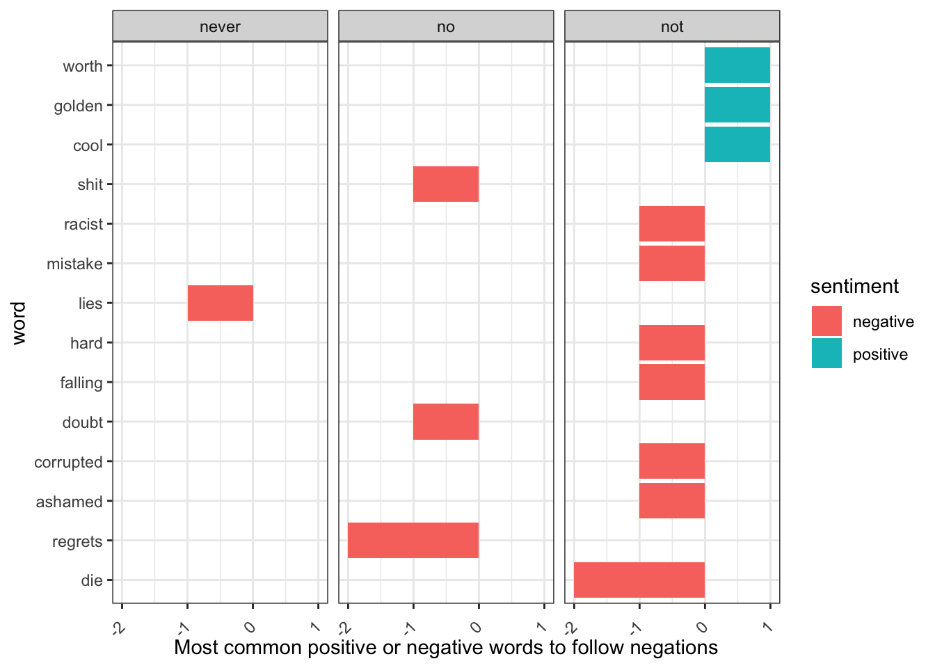
Note: we can see that witout was not plotted as that word did not occur in our dataset. Also as above, look at the words and sentiments: are they correct for the context? Again, always think critically and carefully about your tools and outputs!
9.1.5 Network Visualization of ngrams
We may be interested in visualizing all of the relationships among words simultaneously, rather than just the top few at a time. As one common visualization, we can arrange the words into a network or graph. Here we’ll be referring to a “graph” not in the sense of a visualization, but as a combination of connected nodes. A graph can be constructed from a tidy object since it has three variables:
from: the node an edge is coming from
to: the node an edge is going towards
weight: A numeric value associated with each edge
We will use the igraph package for this.
library('igraph')

# original counts
bigram_counts #using this from before
## # A tibble: 2,191 × 3
## word1 word2 n
## <chr> <chr> <int>
## 1 rshitpost rshitpost 82
## 2 kick punch 24
## 3 <NA> <NA> 24
## 4 ca nt 23
## 5 punch kick 18
## 6 https wwwyoutubecomwatch 17
## 7 season pass 13
## 8 fallout 4 9
## 9 gon na 8
## 10 rocket league 8
## # … with 2,181 more rowsbigram_graph <- bigram_counts %>%
filter(n > 2) %>%
graph_from_data_frame()## Warning in graph_from_data_frame(.): In `d' `NA' elements were replaced with string "NA"bigram_graph## IGRAPH 5d627d0 DN-- 79 49 --
## + attr: name (v/c), n (e/n)
## + edges from 5d627d0 (vertex names):
## [1] rshitpost->rshitpost kick ->punch NA ->NA ca ->nt punch ->kick
## [6] https ->wwwyoutubecomwatch season ->pass fallout ->4 gon ->na rocket ->league
## [11] mario ->kart empty ->bottle mario ->maker nt ->wait punch ->throww
## [16] wo ->nt ben ->dover hit ->chance nt ->understand blue ->shells
## [21] dead ->island holy ->shit jet ->set nt ->apply set ->radio
## [26] wasteland->workshop wedding ->ring 100 ->hit aud ->release barley ->wine
## [31] dark ->souls empty ->bottles empty ->flasks entire ->game front ->page
## [36] hell ->yeah majoras ->mask modding ->community nt ->care nt ->play
## + ... omitted several edgesigraph has inbult plotting functions, but they’re not what the package is designed to do, so many other packages have developed visualization methods for graph objects. So, we will use the ggraph package, because it implements these visualizations in terms of the grammar of graphics, which we are already familiar with from ggplot2.
We can convert an igraph object into a ggraph with the ggraph function, after which we add layers to it, much like layers are added in ggplot2. For example, for a basic graph we need to add three layers: nodes, edges, and text…
library('ggraph')
set.seed(127)

ggraph(bigram_graph, layout = "fr") +
  geom_edge_link() +
  geom_node_point() +
  geom_node_text(aes(label = name), vjust = 1, hjust = 1)
From here, we can see groups of words coming together into pairs and more, for isntance ‘fallout 4’ as a game name, ‘front page’ and ‘jet set ratio’. These can be useful for getting an idea of the themes talked about in a forum. Please note: the data here is a small dataset and you’d normally want a lot more data for these kinds of visualisation.
We can make the network plot better looking by adapting the following:
add the edge_alpha aesthetic to the link layer to make links transparent based on how common or rare the bigram is
add directionality with an arrow, constructed using grid::arrow(), including an end_cap option that tells the arrow to end before touching the node
fiddle with the options to the node layer to make the nodes more attractive (larger, blue points)
add a theme that’s useful for plotting networks, theme_void()
set.seed(127)

a <- grid::arrow(type = "closed", length = unit(.15, "inches"))

ggraph(bigram_graph, layout = "fr") +
  geom_edge_link(aes(edge_alpha = n), show.legend = FALSE,
                 arrow = a, end_cap = circle(.07, 'inches')) +
  geom_node_point(color = "plum2", size = 5) +
  geom_node_text(aes(label = name), vjust = 1, hjust = 1) +
  theme_void()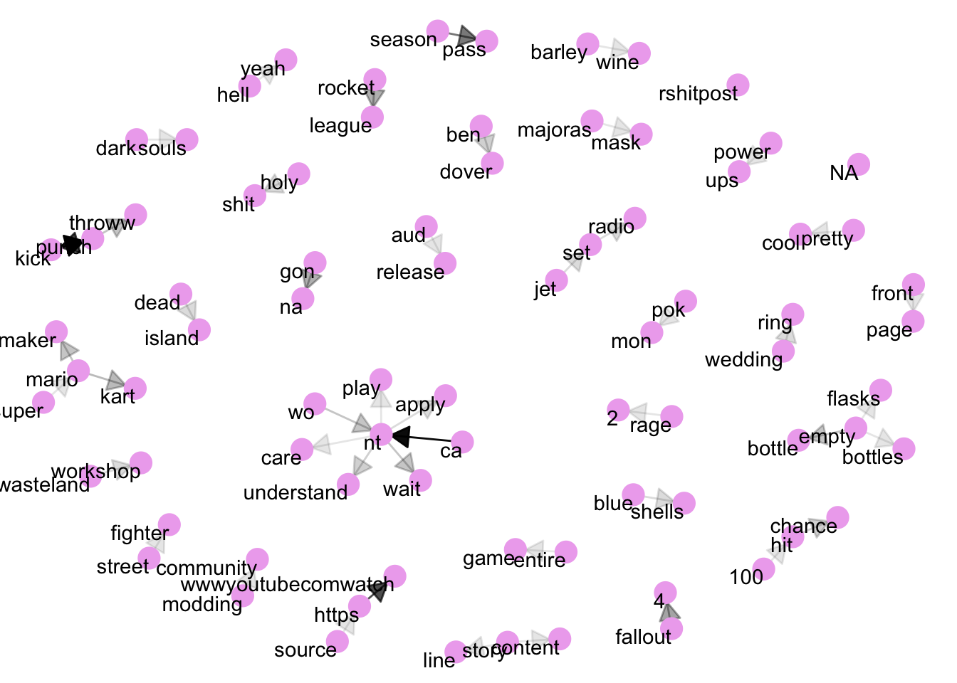
9.1.6 Activity
Part 1: Play with the filtering in the first chunk of code for network visualizations and see how the plot changes when you change the filter level.
Part 2: Rerun all of this analysis using the text_OnlineMSc dataset and practice changing the filters throughout (e.g., when you’re visualising bigrams and you’re filtering, is n>2 enough?)
Part 3: Visualize the network bigram plot for each of the subreddits separately. What differences are there across subreddits?
9.2 Lesson 2: Topic Modelling
In text mining, we often have collections of documents, such as blog posts or news articles, that we’d like to divide into natural groups so that we can understand them separately. Topic modeling is a method for unsupervised classification of such documents, similar to clustering on numeric data, which finds natural groups of items even when we’re not sure what we’re looking for.
Latent Dirichlet allocation (LDA) is a particularly popular method for fitting a topic model. It treats each document as a mixture of topics, and each topic as a mixture of words. This allows documents to “overlap” each other in terms of content, rather than being separated into discrete groups, in a way that mirrors typical use of natural language.
Please note: this is one way to do topic models, there are a number of other packages that do topic modelling so it is worth exploring other methods.
9.2.1 Latent Dirichlet Allocation (LDA)
Latent Dirichlet allocation is one of the most common algorithms for topic modeling.We can understand it as being guided by two principles:
Every document is a mixture of topics. We imagine that each document may contain words from several topics in particular proportions. For example, in a two-topic model we could say: Document 1 is 90% about cats (topic A) and 10% about dogs (topic B), while Document 2 is 30% about cats (topic A) and 70% topic B - dogs.
Every topic is a mixture of words. For example, we could imagine a two-topic model of American news, with one topic for “politics” and one for “entertainment.” The most common words in the politics topic might be “President”, “Congress”, and “government”, while the entertainment topic may be made up of words such as “movies”, “television”, and “actor”. Importantly, words can be shared between topics; a word like “budget” might appear in both equally.
Let’s look at the text_OnlineMSc dataset:
## Warning: Missing column names filled in: 'X1' [1]## Warning: Duplicated column names deduplicated: 'X1' => 'X1_1' [2]##
## ── Column specification ──────────────────────────────────────────────────────────────────────────────────────────────────────────────────────────────────────────────
## cols(
## X1 = col_double(),
## X1_1 = col_double(),
## content = col_character(),
## subreddit = col_character()
## )head(text_OnlineMSc)## # A tibble: 6 × 4
## X1 X1_1 content subreddit
## <dbl> <dbl> <chr> <chr>
## 1 1 53488 <NA> news
## 2 2 53489 protesters lose jobs for not showing up to work arrested for nonpayment news
## 3 3 53490 i do believe they are nt understanding that the phone ca nt be decrypted by apple or anyone news
## 4 4 53491 why did nt they care this much about their freaking home remember all those reporters and camera crews contaminating all that evidence aft… news
## 5 5 53492 even if they wrote a program to stop the wait time or not wipe phone after a certain amount of failed attempts you would still need to get i… news
## 6 6 53493 this is what the fbi was looking for the one terrorist case it can trumpet to prove it needs to unlock anyone s phone at any time news9.2.2 Data Prep and Cleaning
Lets have a look at the LDA() function in the topicmodels package. We first need to do some data cleaning here, where we will remove bits of grammar, convert to lowercase, and also end up creating a document-term matrix, which is the object type required for the LDA() function.
library('tidytext')
news <- na.omit(text_onlineMSc)

#going to get rid of abbreviations etc in text as shown in the function
fix.contractions <- function(doc) {
   doc <- gsub("won't", "will not", doc)
   doc <- gsub("can't", "can not", doc)
   doc <- gsub("n't", " not", doc)
   doc <- gsub("'ll", " will", doc)
   doc <- gsub("'re", " are", doc)
   doc <- gsub("'ve", " have", doc)
   doc <- gsub("'m", " am", doc)
   doc <- gsub("'d", " would", doc)
   doc <- gsub("'s", "", doc)

   return(doc)
}

news$content = sapply(news$content, fix.contractions)


# function to remove special characters throughout the text - so this will be a nicer/easuer base to tokenise and analyse
removeSpecialChars <- function(x) gsub("[^a-zA-Z0-9 ]", " ", x)
news$content = sapply(news$content, removeSpecialChars)

# convert everything to lower case
news$content <- sapply(news$content, tolower)

head(news) #so you can see there is no grammar and everything is in lowercase
## # A tibble: 6 × 3
## X1 content subreddit
## <dbl> <chr> <chr>
## 1 53489 protesters lose jobs for not showing up to work arrested for nonpayment news
## 2 53490 i do believe they are nt understanding that the phone ca nt be decrypted by apple or anyone news
## 3 53491 why did nt they care this much about their freaking home remember all those reporters and camera crews contaminating all that evidence after the… news
## 4 53492 even if they wrote a program to stop the wait time or not wipe phone after a certain amount of failed attempts you would still need to get inside … news
## 5 53493 this is what the fbi was looking for the one terrorist case it can trumpet to prove it needs to unlock anyone s phone at any time news
## 6 53494 the student i did nt want my life to end up as part of a shitty movie like concussion newsNow we need to turn this into a matrix…
news_dtm <- news %>%
  unnest_tokens(word, content) %>%
  anti_join(stop_words) %>% #removing stop words
  dplyr::count(subreddit, word) %>% #this means we have split these data into 3 documents
  #one for each subreddit
  cast_dtm(subreddit, word, n)
## Warning: Outer names are only allowed for unnamed scalar atomic inputs## Joining, by = "word"news_dtm## <<DocumentTermMatrix (documents: 3, terms: 7865)>>
## Non-/sparse entries: 10185/13410
## Sparsity : 57%
## Maximal term length: 129
## Weighting : term frequency (tf)library('topicmodels')
news_lda <- LDA(news_dtm, k = 3, control = list(seed = 127))
news_lda## A LDA_VEM topic model with 3 topics.#note: this is an UNSUPERVISED method, so we have randomly chosen k=3, when
#there might be a better suited number of topics
#we will see what the topics look like and iterate to find
#coherent topics from the data scientist perspective Lets look at the topics more, where we can look at the per-topic-per-word probabilities, β (“beta”):
news_topics <- tidy(news_lda, matrix = "beta")
news_topics
## # A tibble: 23,595 × 3
## topic term beta
## <int> <chr> <dbl>
## 1 1 0 1.41e- 4
## 2 2 0 4.10e- 4
## 3 3 0 1.36e- 4
## 4 1 00 1.41e- 4
## 5 2 00 2.24e- 11
## 6 3 00 1.37e- 4
## 7 1 0080012738255 2.46e-300
## 8 2 0080012738255 3.99e- 12
## 9 3 0080012738255 6.86e- 5
## 10 1 04 3.79e-299
## # … with 23,585 more rows#lets visuaklize these and see what is in here
library('ggplot2')
library('dplyr')
news_top_terms <- news_topics %>%
group_by(topic) %>%
slice_max(beta, n = 15) %>%
ungroup() %>%
arrange(topic, -beta)
news_top_terms %>%
mutate(term = reorder_within(term, beta, topic)) %>%
ggplot(aes(beta, term, fill = factor(topic))) +
geom_col(show.legend = FALSE) +
facet_wrap(~ topic, scales = "free") +
scale_y_reordered() +
theme_bw()
While the removal of stop words has helped here, there are a number of words that are not great (e.g., ‘nt’, ‘http’), which can be added to a list in order to filter out words further. However, the key here is to focus on the topics and whether they make sense: we can see topic 2 mentions names of politicians, whereas topic 3 looks more at money and the police.
When you look at topic model outputs, it is important to carefully consider the words in there and how they come together into a topic, and whether this is the appropriate number. For instance, look here when we re-run this with 6 topics:
news_lda <- LDA(news_dtm, k = 6, control = list(seed = 127))
news_lda
## A LDA_VEM topic model with 6 topics.news_topics <- tidy(news_lda, matrix = "beta")
news_topics## # A tibble: 47,190 × 3
## topic term beta
## <int> <chr> <dbl>
## 1 1 0 1.89e- 4
## 2 2 0 2.09e- 4
## 3 3 0 4.10e- 4
## 4 4 0 8.17e- 5
## 5 5 0 1.44e- 4
## 6 6 0 1.41e- 4
## 7 1 00 1.67e- 4
## 8 2 00 1.16e- 4
## 9 3 00 1.01e-39
## 10 4 00 1.05e- 4
## # … with 47,180 more rowsnews_top_terms <- news_topics %>%
group_by(topic) %>%
slice_max(beta, n = 15) %>%
ungroup() %>%
arrange(topic, -beta)
news_top_terms %>%
mutate(term = reorder_within(term, beta, topic)) %>%
ggplot(aes(beta, term, fill = factor(topic))) +
geom_col(show.legend = FALSE) +
facet_wrap(~topic, scales = "free") +
scale_y_reordered() +
theme_bw()
9.2.3 Activity
Part 1: Do you think the data worked better with 3 or 6 topics? Please discuss in groups of 2-3. What additional data cleaning would you want to do?
Part 2: Play more with this dataset and try different numbers of topics and plotting different numbers of words and find the ideal number of topics from your perspective. What do the topics mean? How do they compare to the rest of the cohort?
Part 3: Rerun the topic models on each of the subreddits separately. What are the topics within each of the subreddits? What is the ideal k? Compare your findings with others.