Chapter 7 Cluster Analysis, part 2
7.1 Lesson 1: Density-based Clustering
Last week we looked at partitioning and hierarchical methods for clustering. In particular, partitioning methods (k-means, PAM, CLARA) and hierarchical clustering are suitable for finding spherical-shaped clusters or convex clusters. Hence, they work well when there are well defiend clusters that are relatively distinct. They also tend to struggle when there are extreme values, outliers, and/or when datasets are noisy.
In contrast, Density-Based Clustering of Applications with Noise (DBScan) is an interesting alternative approach, which is an unsupervised, non-linear algorithm. Rather than focusing entirely on distance between objects/data points, here the focus relates to density. The data is partitioned into groups with similar characteristics or clusters but it does not require specifying the number of clusters for data to be partitioned into. A cluster here, is defined as a maximum set of densely connected points. The bonus of DBSCAN is that can handle clusters of arbitrary shapes in spatial databases with noise.
The goal with DBSCAN is to identify dense regions within a dataset. There are a couple of important parameters for DBSCAN:
epsilon (eps): defines the radius of the neighborhood around a given point
minimum points (MinPts): the minumun number of neighbors within an eps radius
Therefore, if a point has a neighbor count higher than or equal to the MinPts, it is a core point (as in theory this means it will be central to the cluster as it is dense there)… in contrast, if a point has less neighbors than the MinPts, this is a broader point, whereby it is more periheral. Similarly, points can be so far away, they are then deemed noise or an outlier.
Broadly, DBSCAN works as follows:
Randomly select a point p. Retrieve all the points that are density reachable from p (e.g., are within the Maximum radius of the neighbourhood(EPS) and minimum number of points within eps neighborhood(Min Pts))
Each point, with a neighbor count greater than or equal to MinPts, is marked as core point or visited.
For each core point, if it’s not already assigned to a cluster, create a new cluster. Find recursively all its density connected points and assign them to the same cluster as the core point
Iterate through the remaining unvisited points in the dataset
Lets have a go. We will use the multishapes dataset from the factoextra package:
library('factoextra')

data("multishapes")
df <- multishapes[,1:2] #removing the final column using BASE R which is the cluster label

plot(df$x, df$y) #to show you what this data looks like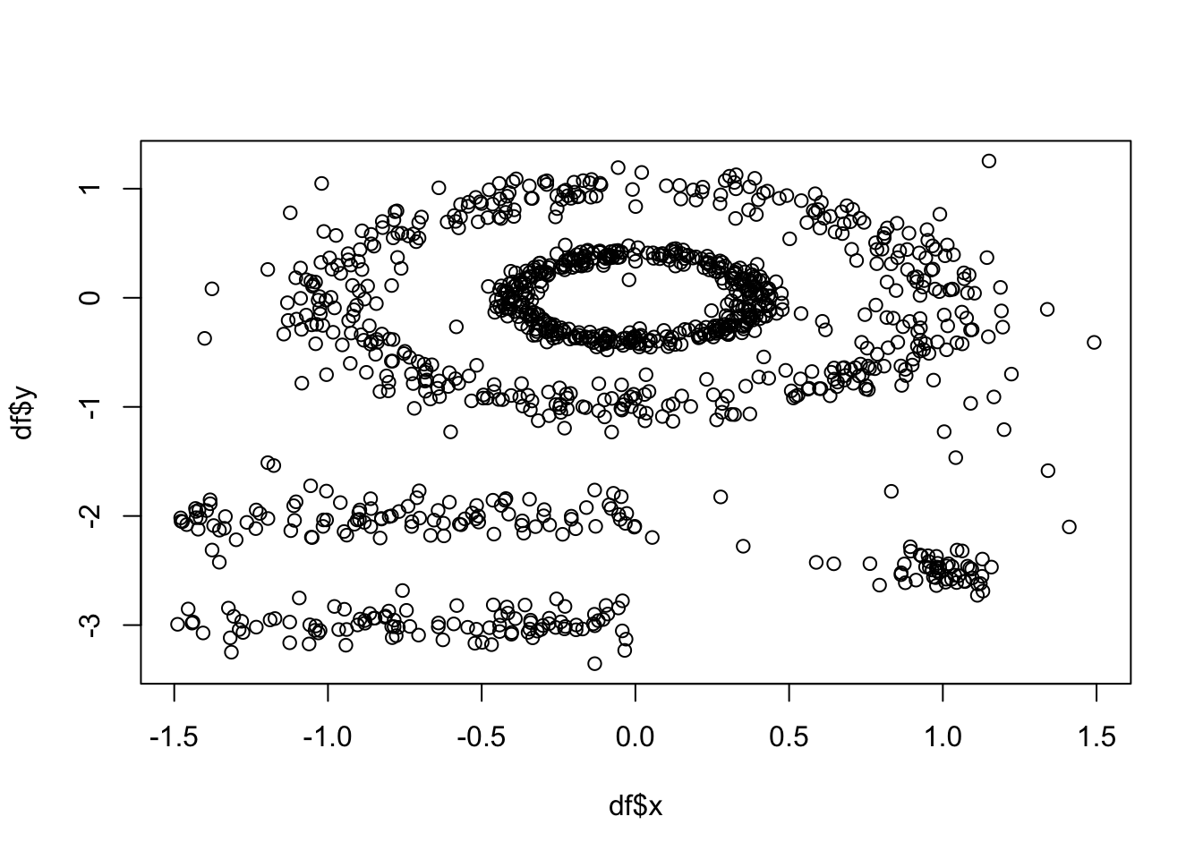
As above, k-means (among other partitioning algorithms) are not great at identifying objects that are non-spherical. So, lets quickly see how k-means handles these data. We can see there are 5 clusters, so we wil proceed with k=5.
set.seed(127)
km.res <- kmeans(df, 5, nstart = 25)
fviz_cluster(km.res, df,ellipse.type = "point",
geom=c("point"),
palette = "jco",
ggtheme = theme_classic())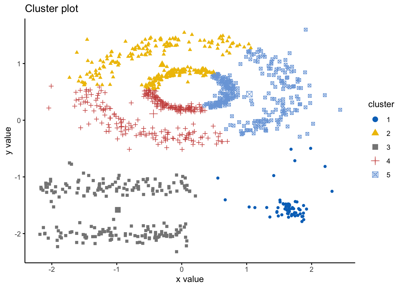 As we can see here, the k-means has indeed spliced the data and found 5 clusters, however, it ignores the spaces between clusters that we would expect. Hence, this is where DBSCAN is an alternative way to mitigate these issues. Here we will use the DBSCAN package and the fpc package and the dbscan() command. The simple format of the command dbscan() is as follows: dbscan(data, eps, MinPts, scale = F, method = ““); where: data is the data as a datafreame, matrix, or dissimiliarity matric via the dist() function; eps is the reachability maximum distance, MinPts is the reachability minimum number of points, scale - if true means the data will be scaled, method can be”dist” where it treats data as a raw matrix, “raw” where it is treated as raw data, and “hybrid” where it expects raw data but calculates partial distance matrices. Note that the plot.dbscan() command uses different points for outliers.
We said above that DBSCAN algorithm requires users to specify the optimal eps values and the parameter MinPts. However, how do we know what those values should be? Well, there are ways! It is important to note that a limitation of DBSCAN is that it is sensitive to the choice of epsilon, in particular if clusters have different densities.
If the epsilon value is too small, sparser clusters will be defined as noise. If the value chosen for the epsilon is too large, denser clusters may be merged together. This implies that, if there are clusters with different local densities, then a single epsilon value may not suffice…So what do we do? Well, a common way is to compute the k-nearest neighbours distances, where we can use this to calculate the average distance to every point to its nearest neighbors. Here, the value of k will be specified by the data scientist/analyst and will be the MinPts value. We will produce an almost inverse elbow plot (like with k-means), known as a knee plot, where we want point where there is a sharp bend upwards as our eps value.
Lets have a look:
library('fpc')
library('dbscan')

dbscan::kNNdistplot(df, k =  5)

#so we can see that the knee is around 0.15 (as seen on the dotted line)
dbscan::kNNdistplot(df, k =  5) +
  abline(h = 0.15, lty = 2)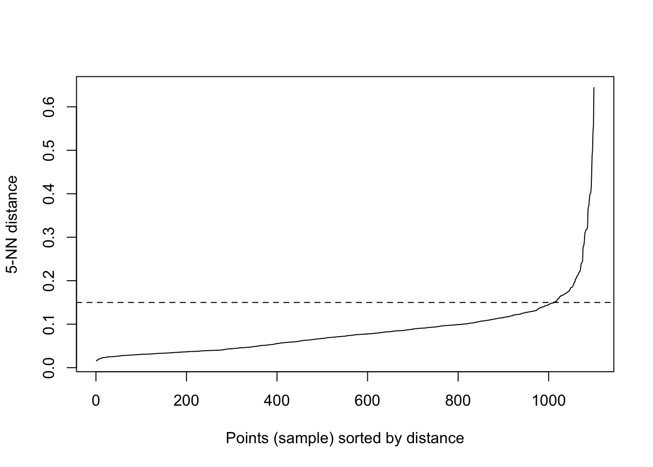
## integer(0)So, lets use these values and run the dbscan algorithm:
# Compute DBSCAN using fpc package
set.seed(127)

db <- fpc::dbscan(df, eps = 0.15, MinPts = 5)

# Plot DBSCAN results
plot(db, df, main = "DBSCAN", frame = FALSE)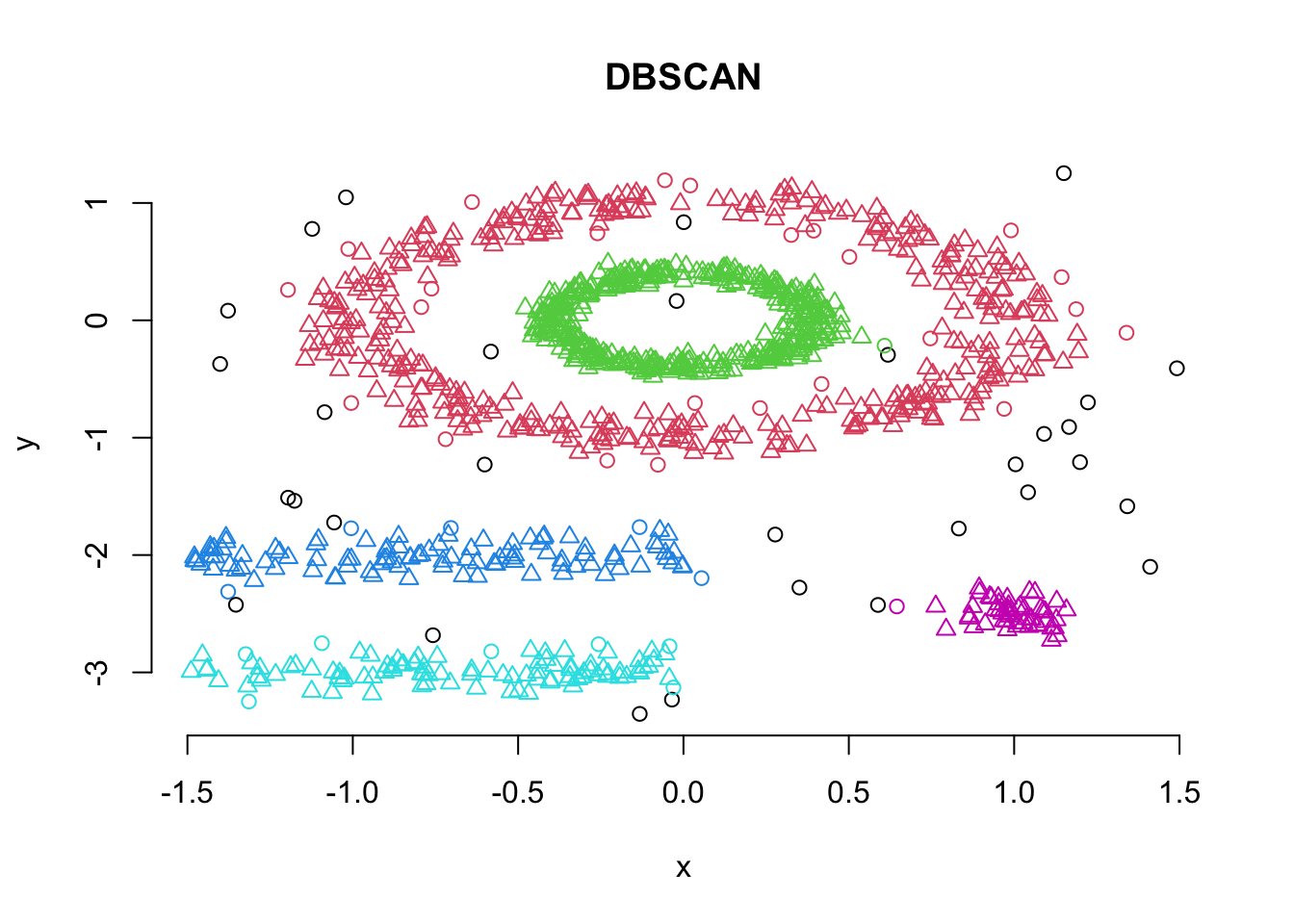
#also visualising the fiz_cluster, too:
fviz_cluster(db, df,ellipse.type = "point",
geom=c("point"),
palette = "jco",
ggtheme = theme_classic())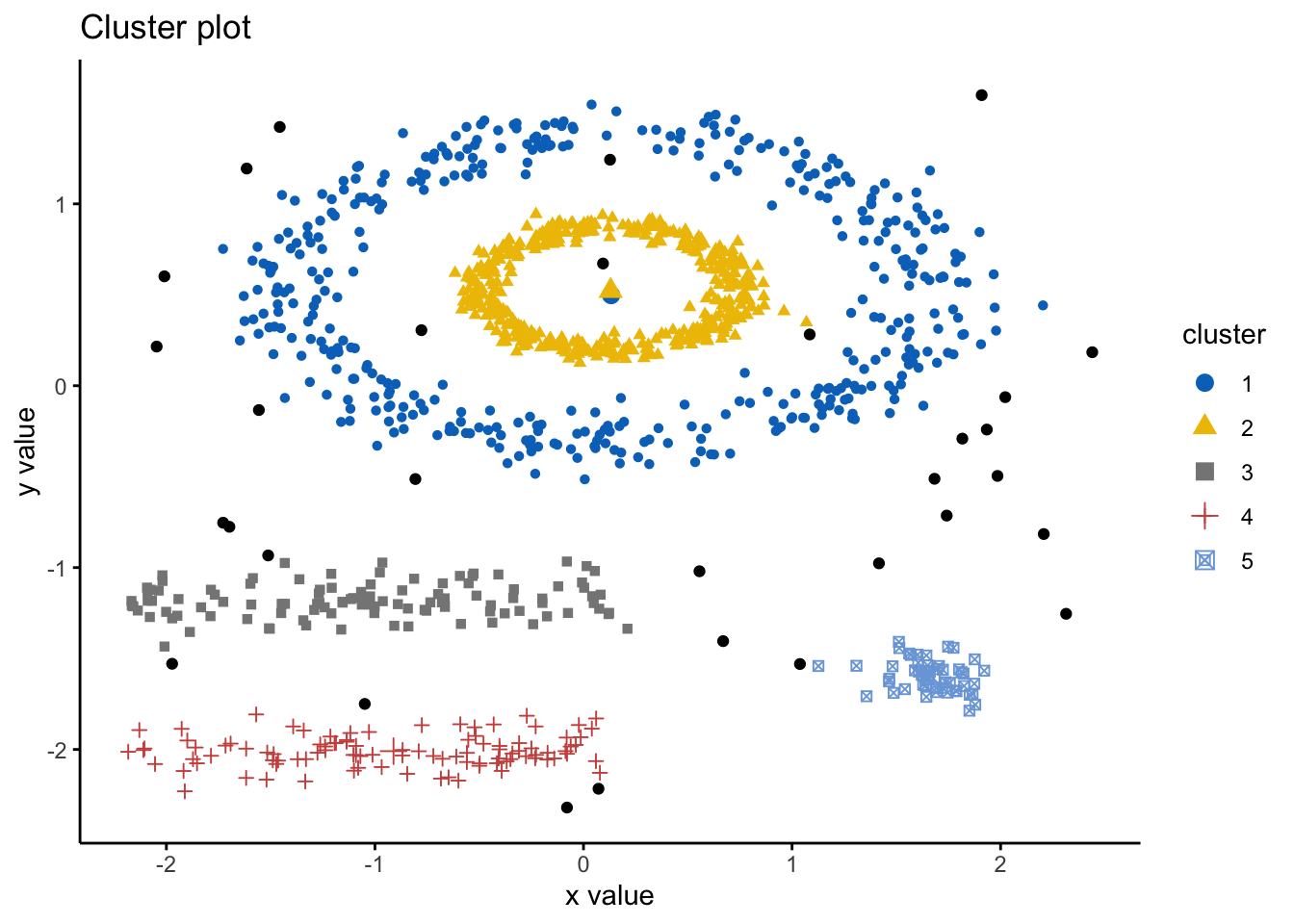 We can look at the numerical results by printing db:
print(db)## dbscan Pts=1100 MinPts=5 eps=0.15
## 0 1 2 3 4 5
## border 31 24 1 5 7 1
## seed 0 386 404 99 92 50
## total 31 410 405 104 99 51Note here that cluster 0 refers to the outliers.
7.1.1 Activity
Part 1: Using the multishapes dataset, try different values for eps and MinPts: what happens to the results when you change these?
Part 2: Try running the dbscan algorithm on the iris dataset, how do the results differ from the partitioning and hierarchial algorithm results?
7.2 Lesson 2: Soft Clustering
As introduced before, there are two types of clustering: hard and soft. The methods we have looked at are types of hard clustering whereby a point is assigned to only one cluster. However, soft clustering, also known as fuzzy clustering, is where each point is assigned a probability of belonging to each cluster. Hence, each cluster will have a membership coefficient that is the degree to which they belong to a given cluster. So, in fuzzy clustering, the degree to which an element belongs to a given cluster, is a numerical value varying from 0 to 1. One of the most common methods is the fuzzy c-means (FCM) algorithm. The centroid of a cluster is calculated as the mean of all points, weighted by their degree of belonging to the cluster.
To do this, we can use the function fanny() from the cluster package, which takes this format: fanny(data, k, metric, stand), where data is a dataframe or matrix, or similiarity matrix from the dist() command, k is the number of clusters, metric is the method for calculating similarities between points, and stand if true is where data are standardized before computing similarities.
Here, we will output membership as a matrix containing the degree to which each point belongs to each cluster, coeff as Dunn’s partition coefficient. We are given also the normalized form of this coefficient, which has a value between 0-1. A low value of Dunn’s coefficient indicates a very fuzzy clustering, whereas a value close to 1 indicates a near-crisp clustering, and finally, we also are given clustering and this is a vector of the nearest crisp grouping of points.
Lets use the iris dataset and try this:
library('cluster')

df <- iris #loading data

df <- dplyr::select(df,
                    -Species) #removing Species

df <- scale(df) #scaling

head(df)
## Sepal.Length Sepal.Width Petal.Length Petal.Width
## [1,] -0.8976739 1.01560199 -1.335752 -1.311052
## [2,] -1.1392005 -0.13153881 -1.335752 -1.311052
## [3,] -1.3807271 0.32731751 -1.392399 -1.311052
## [4,] -1.5014904 0.09788935 -1.279104 -1.311052
## [5,] -1.0184372 1.24503015 -1.335752 -1.311052
## [6,] -0.5353840 1.93331463 -1.165809 -1.048667Lets now compute the soft clustering and wew will also inspect the membership, coeff, and clustering results
res.fanny <- fanny(df, 3) #as we know k=3 here, we will use that

head(res.fanny$membership, 20) # here we can look at the first 20  memberships
## [,1] [,2] [,3]
## [1,] 0.8385968 0.07317706 0.08822614
## [2,] 0.6704536 0.14154548 0.18800091
## [3,] 0.7708430 0.10070648 0.12845057
## [4,] 0.7086764 0.12665562 0.16466795
## [5,] 0.8047709 0.08938753 0.10584154
## [6,] 0.6200074 0.18062228 0.19937035
## [7,] 0.7831685 0.09705901 0.11977247
## [8,] 0.8535825 0.06550752 0.08090996
## [9,] 0.5896668 0.17714551 0.23318765
## [10,] 0.7289922 0.11770684 0.15330091
## [11,] 0.7123072 0.13395910 0.15373372
## [12,] 0.8306362 0.07568357 0.09368018
## [13,] 0.6703940 0.14236702 0.18723902
## [14,] 0.6214078 0.16611879 0.21247344
## [15,] 0.5557920 0.21427105 0.22993693
## [16,] 0.4799971 0.25653355 0.26346938
## [17,] 0.6276064 0.17692368 0.19546993
## [18,] 0.8367988 0.07391816 0.08928306
## [19,] 0.6053432 0.18726365 0.20739316
## [20,] 0.7037729 0.13851778 0.15770936res.fanny$coeff #looking at the Dunns partition coefficients ## dunn_coeff normalized
## 0.4752894 0.2129341head(res.fanny$clustering, 20) #looking at the groups as the first 20 points## [1] 1 1 1 1 1 1 1 1 1 1 1 1 1 1 1 1 1 1 1 1Of course, as always, we can visualize this using the factoextra package!
#note you can change the ellipse type from point, convex, norm, among others
# try them out!
fviz_cluster(res.fanny, df,ellipse.type = "norm",
             geom=c("point"),
             palette = "jco",
             ggtheme = theme_classic())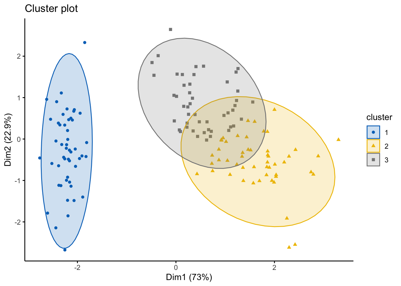
7.2.1 Activity
Try the soft clustering algorithm on the diamonds, mpg, and also the multishapes dataset. Discuss you results in groups of 2-3.
7.3 Lesson 3: Evaluation Techniques
When doing any machine learning and data analytics it is important to pause, reflect, and consider how well our analysis fits with the data. This is particularly important with UNsupervised learning, such as clustering, as of course, we –the data scientist/analyst–are the ones who need to interpret these clusters. While it is relatively simple for the datasets we have used here as with the iris dataset, we know the species that the points will generally cluster into. However, this is often not what would happen when you’re using clustering in practice will be. It is more likely you’ll be given a dataset with a variety of metrics and you have no idea what the naturally occurring clusters will be, and therefore, the interpretation is critical.
For instance, if you had heart rate from a wearable device, what could you realistically infer from this if we notice a cluster had particularly high heart rates? Well, it depends… on what the other data are and the context. This might mean they were exercising hard when those measurements were taken, it might mean they are stressed if they were on a phonecall when the measurement was taken, it might infer an underlying health condition. Hence, we must be extremely careful with how we interpret and what biases we bring when analyzing these data. Again, if we had a dataset where we had information about how much someone uses their smartphone, and there is a cluster with ‘high’ smartphone usage–what do we infer? They use their phone too much? What about people who use phones for work and therefore are taking a lot of calls or answering emails on the device? Context and understanding your data are key, alongside knowing what questions you want to answer are.
Other than visual inspection via the plots we have created and also interpreting the clusters and thinking ‘do these clusters make sense?’, there are other statistics and diagnostics we can do in R that will help us also understand whether the clusters are appropriate. However, it is important that the human interpretation is key.
7.3.1 Internal Clustering Validation Methods
Remember here, the goal of clustering is to minimize the average distance within clusters; and to maximize the average distance between clusters. Therefore, some measures we can conisider to evaluate our clustering output are:
Compactness measures: to evaluate how close objects are within clusters, whereby low within-cluster variation implies good clustering
Separation measures: to determine how well separated a cluster is from another, which can be the distance between cluster centers, and pairwise minimum distances between objects in each cluster
Connectivity measures: relates to the nearest neighbors within clusters
The first way we can look at this is by running a Silhouette Analysis. This analysis measures how well an observation is clustered and it estimates the average distance between clusters. The silhouette plot displays a measure of how close each point in one cluster is to points in the neighboring clusters. Essentially, clusters with a large silhouette width are well very clustered, those with width near 0 mean the observation lies between two clusters, and negative silhouette widths mean the observation is likely in the wrong cluster.
We can run this analysis using the silhouette() function in the cluster package, as follows: silhouette(x, dist), where x is a vector of the assigned clusters, and the dist is the distance matrix via the dist() funciton. We will be returned an object that has the cluster assignment of each observation, the neighbour of the cluster, and the silhouette width.
We will use the iris dataset:
library('cluster')

df <- iris #loading data
df <- dplyr::select(df,
                    -Species) #removing Species
df <- scale(df) #scaling
head(df)
## Sepal.Length Sepal.Width Petal.Length Petal.Width
## [1,] -0.8976739 1.01560199 -1.335752 -1.311052
## [2,] -1.1392005 -0.13153881 -1.335752 -1.311052
## [3,] -1.3807271 0.32731751 -1.392399 -1.311052
## [4,] -1.5014904 0.09788935 -1.279104 -1.311052
## [5,] -1.0184372 1.24503015 -1.335752 -1.311052
## [6,] -0.5353840 1.93331463 -1.165809 -1.048667# lets run a quick K-means algo
km.res <- eclust(df, "kmeans", k = 3,
nstart = 25, graph = FALSE)
#running the silhouette analysis
sil <- silhouette(km.res$cluster, dist(df))
head(sil[, 1:3], 10) #looking at the first 10 observations## cluster neighbor sil_width
## [1,] 1 2 0.7341949
## [2,] 1 2 0.5682739
## [3,] 1 2 0.6775472
## [4,] 1 2 0.6205016
## [5,] 1 2 0.7284741
## [6,] 1 2 0.6098848
## [7,] 1 2 0.6983835
## [8,] 1 2 0.7308169
## [9,] 1 2 0.4882100
## [10,] 1 2 0.6315409#we can create an pretty visual of this
library('factoextra')
fviz_silhouette(sil)## cluster size ave.sil.width
## 1 1 50 0.64
## 2 2 53 0.39
## 3 3 47 0.35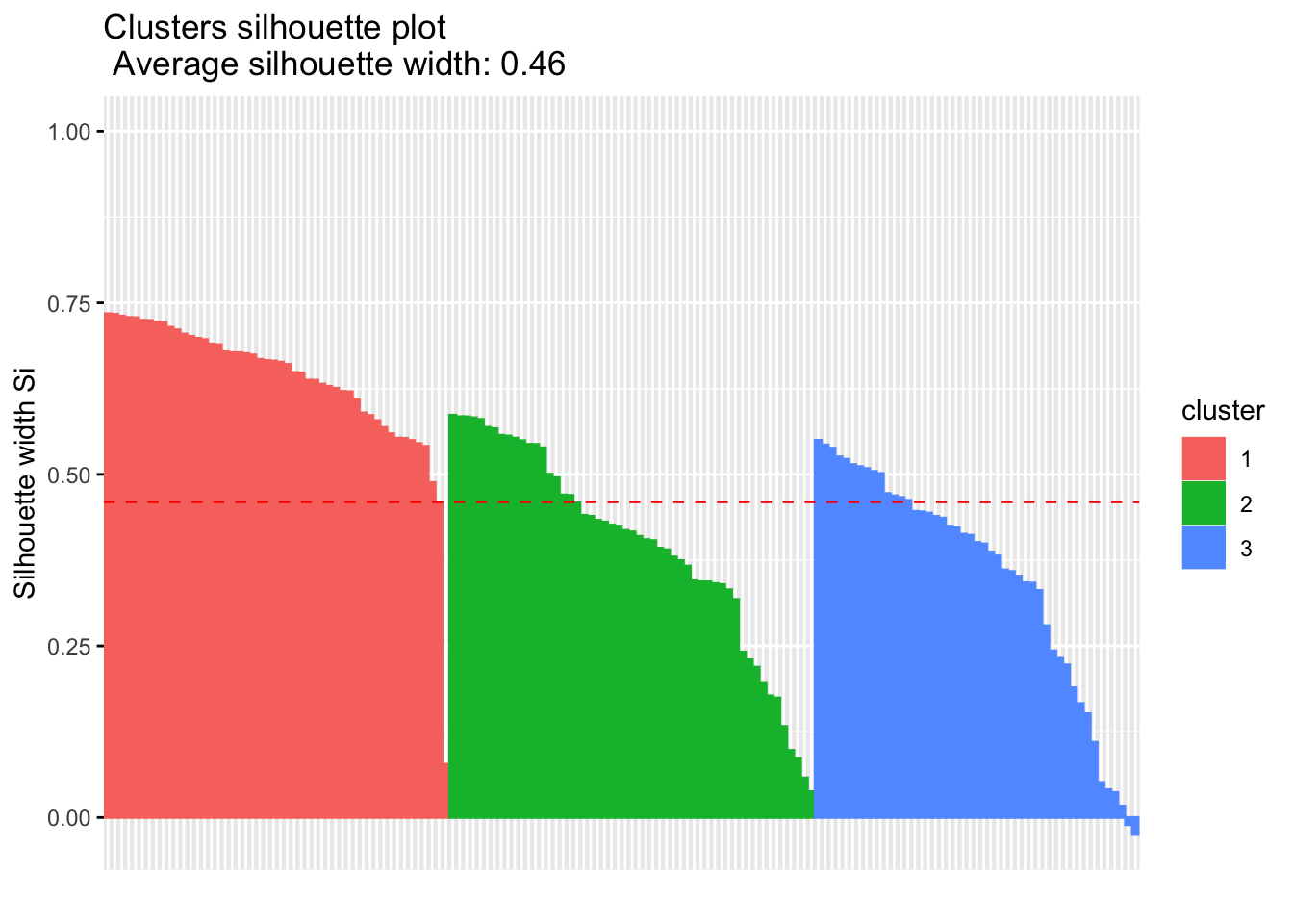
We can look at the results of this analysis as follows:
# Summary of silhouette analysis
si.sum <- summary(sil)
# Average silhouette width of each cluster
si.sum$clus.avg.widths
## 1 2 3
## 0.6363162 0.3933772 0.3473922What about the negative silhouette coefficients? This means that these observations may not be in the right cluster. Lets have a look at these samples and inspect them further:
# Silhouette width of observation
sil <- km.res$silinfo$widths[, 1:3]
# Objects with negative silhouette
neg_sil_index <- which(sil[, 'sil_width'] < 0)
sil[neg_sil_index, , drop = FALSE]## cluster neighbor sil_width
## 112 3 2 -0.01058434
## 128 3 2 -0.02489394There are a few options, where typically if there were many observations, we might need to try different values for k on the clustering algorithm, or we might reassign these observations to another cluster and examine whether this improves the performance.
Another metric we can use to evaluate clusters is the Dunn Index, which should be familiar… Essentially, if the data set contains compact and well-separated clusters, the diameter of the clusters is expected to be small and the distance between the clusters is expected to be large. Hence, Dunn index should be maximized. This can be done using the cluster.stats() command in the fpc package as follows: cluster.stats(d, clustering, al.clustering = NULL), where d is a distance matrix from the dist() function, clustering is the vector of clusters for each data point, and alt.clustering is a vector for clustering, indicating an alternative clustering.
Please note, the cluster.stats() command also has wide capabilities, where we can look at a number of other statistics:
cluster.number: number of clusters
cluster.size: vector containing the number of points within each cluster
average.distance, median.distance: vector containing the cluster-wise within average/median distances
average.between: average distance between clusters. (this would be as large as possible)
average.within: average distance within clusters. (this should be as small as possible)
clus.avg.silwidths: vector of cluster average silhouette widths (this should be as close to 1 as possible, and no negative values)
within.cluster.ss: a generalization of the within clusters sum of squares (k-means objective function)
dunn, dunn2: Dunn index
corrected.rand, vi: Two indexes to assess the similarity of two clustering: the corrected Rand index and Meila’s VI
Let’s look at this closer using the scaled iris dataset from before:
library('fpc')
# Compute pairwise-distance matrices
df_stats <- dist(df, method ="euclidean")
# Statistics for k-means clustering
km_stats <- cluster.stats(df_stats, km.res$cluster) #this is using the kmeans clustering we did for the silhouette
km_stats #this prints all the statistics## $n
## [1] 150
##
## $cluster.number
## [1] 3
##
## $cluster.size
## [1] 50 53 47
##
## $min.cluster.size
## [1] 47
##
## $noisen
## [1] 0
##
## $diameter
## [1] 5.034198 2.922371 3.343671
##
## $average.distance
## [1] 1.175155 1.197061 1.307716
##
## $median.distance
## [1] 0.9884177 1.1559887 1.2383531
##
## $separation
## [1] 1.5533592 0.1333894 0.1333894
##
## $average.toother
## [1] 3.647912 2.674298 3.081212
##
## $separation.matrix
## [,1] [,2] [,3]
## [1,] 0.000000 1.5533592 2.4150235
## [2,] 1.553359 0.0000000 0.1333894
## [3,] 2.415024 0.1333894 0.0000000
##
## $ave.between.matrix
## [,1] [,2] [,3]
## [1,] 0.000000 3.221129 4.129179
## [2,] 3.221129 0.000000 2.092563
## [3,] 4.129179 2.092563 0.000000
##
## $average.between
## [1] 3.130708
##
## $average.within
## [1] 1.224431
##
## $n.between
## [1] 7491
##
## $n.within
## [1] 3684
##
## $max.diameter
## [1] 5.034198
##
## $min.separation
## [1] 0.1333894
##
## $within.cluster.ss
## [1] 138.8884
##
## $clus.avg.silwidths
##         1         2         3
## 0.6363162 0.3933772 0.3473922
##
## $avg.silwidth
## [1] 0.4599482
##
## $g2
## NULL
##
## $g3
## NULL
##
## $pearsongamma
## [1] 0.679696
##
## $dunn
## [1] 0.02649665
##
## $dunn2
## [1] 1.600166
##
## $entropy
## [1] 1.097412
##
## $wb.ratio
## [1] 0.3911034
##
## $ch
## [1] 241.9044
##
## $cwidegap
## [1] 1.3892251 0.7824508 0.9432249
##
## $widestgap
## [1] 1.389225
##
## $sindex
## [1] 0.3524812
##
## $corrected.rand
## NULL
##
## $vi
## NULL7.3.2 External Clustering Validation Method
Sometimes we might have data that we can compare results (hence, external validation), for instance the iris dataset has the species label we clustered. Hence, we can compare the clustering outputs and the species label already in the dataset. Note: we will not always have this, so this is not always possible.
So, using our kmeans clustering above, lets compare against the original iris dataset labels:
table(iris$Species, km.res$cluster)##
## 1 2 3
## setosa 50 0 0
## versicolor 0 39 11
## virginica 0 14 36So, lets interpret this:
All setosa species (n = 50) has been classified in cluster 1
A large number of versicor species (n = 39 ) has been classified in cluster 3, however, some of them ( n = 11) have been classified in cluster 2
A large number of virginica species (n = 36 ) has been classified in cluster 2, however, some of them (n = 14) have been classified in cluster 3
This shows there is some misclassifcation between clusters due to lack of distinctive features. Hence, we might want to try different clustering methods IF our question relates to whether we can cluster according to species.
7.3.3 Activity
Part 1: conduct a silhouette analysis using the iris dataset for ouputs from the
PAM algorithm
Hierarchical algorithms (both agglomerative and divisive)
Part 2: From the outputs above, how well do the clusters fit the original species data (species)?