Chapter 8 Text Mining, part 1
8.1 Lesson 1: Introduction to Text Mining
Text mining (also known as text analytics) in its simplest form, is a method for helping understand meaning and context from a (large) amounts of text. Essentially, it is a set of methods for structuring information from unstructured text. For instance, via text mining tools we have (hopefully) less spam in our inboxes and abilities to start to understand sentiment in social media data.
Broadly speaking, the overarching goal of text mining is to turn text into data so that it is suitable for other forms of analysis, so we sometimes convert words into vectors. To achieve this, there is a need for applying often computationally-intensive algorithms and statistical techniques to text documents. There are a number of types of text analysis, including:
Information Retrieval (IR) – Retrieval of text documents via text summarization or information extraction to extract the useful information for the user (e.g., search engines)
Information Extraction (IE) – Extraction of useful information from text (e.g., identification of entities, events, relationships from semi- or unstructured text)
Categorization – Supervised learning to categorize documents (e.g., spam filtering, automatic detection of genre…)
Clustering – Unsupervised process, where documents are allocated into clusters (e.g., pattern recognition); can be a stand-alone tool or a pre-processing step
Summarization – Automatically create a useful compressed version of the text
Please note: many of these are entire fields in their own right and are highly complex, so this course will show you how to clean and process textual data, which makes up for most of the analytics pipelines, alongside some sentiment analysis, term-frequency insights, n-grams, and unsupervised techniques (e.g., topic modeling).
Before we start, lets cover some definitionsas this will come up throughout this and next week’s content:
Document: some text; e.g., blog posts, tweets, comments
Corpus: objects that typically contain raw strings (pre-tokenized) annotated with additional metadata (e.g., ID, date/time, title, language)
String: raw character vectors (e.g., ‘hello, world’)
Document-term matrix (DTM): sparse matrix describing a collection (or corpus) of documents, where:
- Each row = a document
- Each column = a term
- Each value = typically frequency of term (or tf-idf)
Parsing, which is the process of analyzing text made of a sequence of tokens to determine some structure or rules of a formal grammar. ‘Parsing’ comes from Latin pars (orationis) meaning part (of speech). Parsing usually applies to text – aka, reading text and converting it into a more useful in-memory format (e.g., parsing errors in earlier lectures). For example, an HTML parser will take the sequence of characters (or bytes) and convert them into elements, attributes.
Tokenization is the process of converting any text or sequence of characters into tokens
- These are strings that can be: words, phrases, symbols…
- During this process, we want the data to be as clean as possible, where we might remove punctuation (among other types of words, like stop words)
Text Normalization tends to occur before tokenization, but this is an iterative process, where you clean and normalize your text and then run some analysis post-tokenization and see an anomaly, and go back to re-clean and re-normalize your text… this might include:
- Removing punctuation
- Converting all text to lowercase
- Stemming, which is where you remove the back end of a word to get the ‘stem’, e.g., running, runs, ran, and runner become run
- Handling typing errors
- Use of regular expressions (regex) to remove (or find) unnecessary text strings (e.g., symbols in social media data)
- Handling different languages
Regular Expressions are extremely powerful functions for pattern matching. They are concise and flexible, where you might want to remove all numbers from some text and you’d use a regex and call [[:digit:]], which would match numbers and remove them.
For this course, we will follow the ‘Tidy Text Way’ (https://www.tidytextmining.com/tidytext.html), where the large online resource is freely available too. What do we mean by this? Well, tidy data has a specific structure:
Each variable is a column
Each observation is a row
Each type of observational unit is a table
Therefore, the tidy text format as being a table with one-token-per-row. A token is a meaningful unit of text, such as a word, that we are interested in using for analysis, and tokenization is the process of splitting text into tokens. This one-token-per-row structure is in contrast to the ways text is often stored in current analyses, perhaps as strings or in a document-term matrix. For tidy text mining, the token that is stored in each row is most often a single word, but can also be an n-gram, sentence, or paragraph. In the tidytext package, we provide functionality to tokenize by commonly used units of text like these and convert to a one-term-per-row format.
Let’s have a look…we will import the reddit data, specifically pulled from r/gaming
##
## ── Column specification ──────────────────────────────────────────────────────────────────────────────────────────────────────────────────────────────────────────────
## cols(
##   content = col_character(),
##   id = col_character(),
##   subreddit = col_character()
## )library('dplyr')
library('stringr')
library('tidytext')
library('tm')
head(gaming_subreddit) #so here the bit we will work on is 'content'## # A tibble: 6 × 3
## content id subreddit
## <chr> <chr> <chr>
## 1 you re an awesome person 464s… gaming
## 2 those are the best kinds of friends and you re an amazing friend for getting him that kudos to both of you 464s… gaming
## 3 <NA> 464s… gaming
## 4 <NA> 464s… gaming
## 5 holy shit you can play shuffle board in cod 464s… gaming
## 6 implemented a ban system for players who alter game files to give unfair advantage in online play how about giving us the option to opt of this sh… 464s… gamingFrom here, we want to tokenize the content. This function uses the tokenizers package to separate text in the original data frame into tokens. The default tokenizing is for words, but other options include characters, n-grams, sentences, lines, paragraphs, or separation around a regex pattern that you can specify in the unnest_tokens(x, y) command. Here, we will use words only – as denoted by word being used below:
tidy_data <- gaming_subreddit %>%
    unnest_tokens(word, content)

head(tidy_data) #where you can see the last column as 'word' which
## # A tibble: 6 × 3
## id subreddit word
## <chr> <chr> <chr>
## 1 464sjk gaming you
## 2 464sjk gaming re
## 3 464sjk gaming an
## 4 464sjk gaming awesome
## 5 464sjk gaming person
## 6 464sjk gaming those#as tokenized the entire datasetNow we have the data into a tidytext friendly format, we can manipulate this with tidy tools like dplyr. As we talked about above, we will want to remove stop words; stop words are words that are not useful for an analysis, typically extremely common words such as “the”, “of”, “to”, and so forth in English. We can remove stop words (kept in the tidytext dataset stop_words) with an anti_join():
data(stop_words)

head(stop_words) #so you can see the stop words here
## # A tibble: 6 × 2
## word lexicon
## <chr> <chr>
## 1 a SMART
## 2 a's SMART
## 3 able SMART
## 4 about SMART
## 5 above SMART
## 6 according SMART#sometimes you need to make your own list
tidy_data <- tidy_data %>%
anti_join(stop_words)## Joining, by = "word"#notice how the dataframe tidy_books went from 20,670 rows
# to 7,889 rows after removing stop wordsSo, lets start looking at this data! We can count the words and see which are the most common words and visualize this:
tidy_data %>%
  dplyr::count(word, sort = TRUE) #using dplyr to count
## # A tibble: 3,346 × 2
## word n
## <chr> <int>
## 1 game 162
## 2 nt 152
## 3 <NA> 97
## 4 rshitpost 83
## 5 play 57
## 6 http 44
## 7 time 44
## 8 people 40
## 9 games 39
## 10 shit 39
## # … with 3,336 more rows#we could also use tally() here
#note here the large number of NA (e.g., empty rows)
tidy_data %>%
dplyr::count(word, sort = TRUE) %>%
filter(n > 20) %>%
mutate(word = reorder(word, n)) %>%
ggplot(aes(n, word)) +
geom_col() +
labs(y = NULL)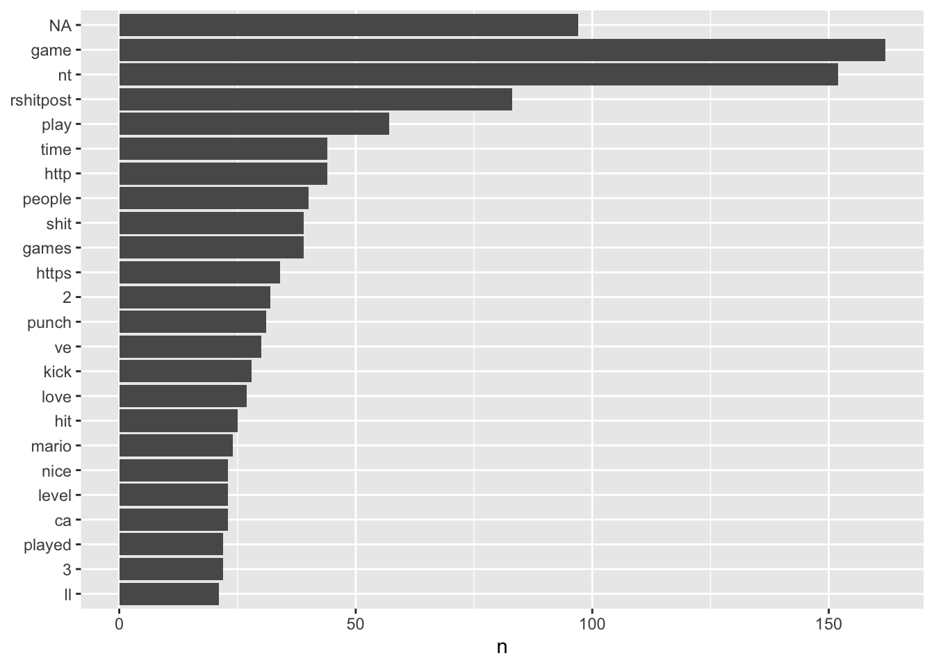
There are a few things to notice here. First, the NA – aka, empty rows. This is an intersting artefact in the data, where no words were captured when these data were scraped, therefore, we need to consider what to do here (it is perhaps likely this was a meme or photo only, hence does not appear in the dataset). Second, there are words like http, https, ca, and 3, which may not be useful. So, these can also be filtered out by removing NA values.
tidy_data <- na.omit(tidy_data) #removing NA values

tidy_data %>%
  dplyr::count(word, sort = TRUE) %>% #counting
  filter(n > 20) %>% #removing any words that have appears <20 times
  mutate(word = reorder(word, n)) %>% #reordering words so they plot in order
  ggplot(aes(n, word)) + #plot
  geom_col() +
  labs(y = NULL)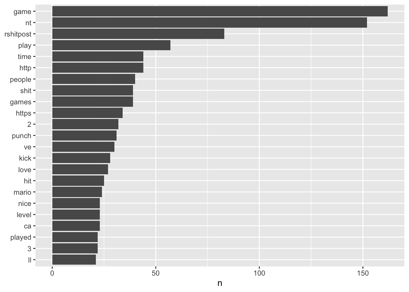
We could look at the top words used by each of the users in the dataset by grouping by id.
library('forcats')

top_words_id <- tidy_data %>%
    dplyr::count(id, word, sort = TRUE) %>%
    group_by(id) %>% #so we are grouping by user here
#keeps top 15 words by each user
    top_n(15) %>%
    ungroup() %>%
# Make the words an ordered factor so they plot in order using forcats
    mutate(word = fct_inorder(word))
## Selecting by nhead(top_words_id)## # A tibble: 6 × 3
## id word n
## <chr> <fct> <int>
## 1 d02qkvw rshitpost 83
## 2 d02qkvw nt 36
## 3 d02qkvw game 31
## 4 d02i70v punch 29
## 5 d02mmay game 29
## 6 d02i70v kick 27We can visualize this nicely too, using facet_wrap, which allows us to have a separate plot for each user:
ggplot(top_words_id, aes(y = fct_rev(word), x = n, fill = id)) +
  geom_col() +
  guides(fill = FALSE) +
  labs(y = "Count", x = NULL,
       title = "15 most frequent words used by reddit r/gaming users") +
  facet_wrap(vars(id), scales = "free_y") +
  theme_bw()
## Warning: `guides(<scale> = FALSE)` is deprecated. Please use `guides(<scale> = "none")` instead.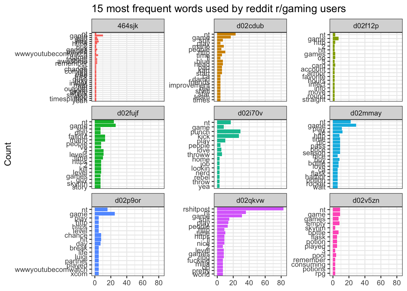
There are a number of other things we can do before getting into other text mining. For instance, word clouds:
library('wordcloud')

tidy_data %>%
  dplyr::count(word) %>%
  with(wordcloud(word, n, max.words = 100))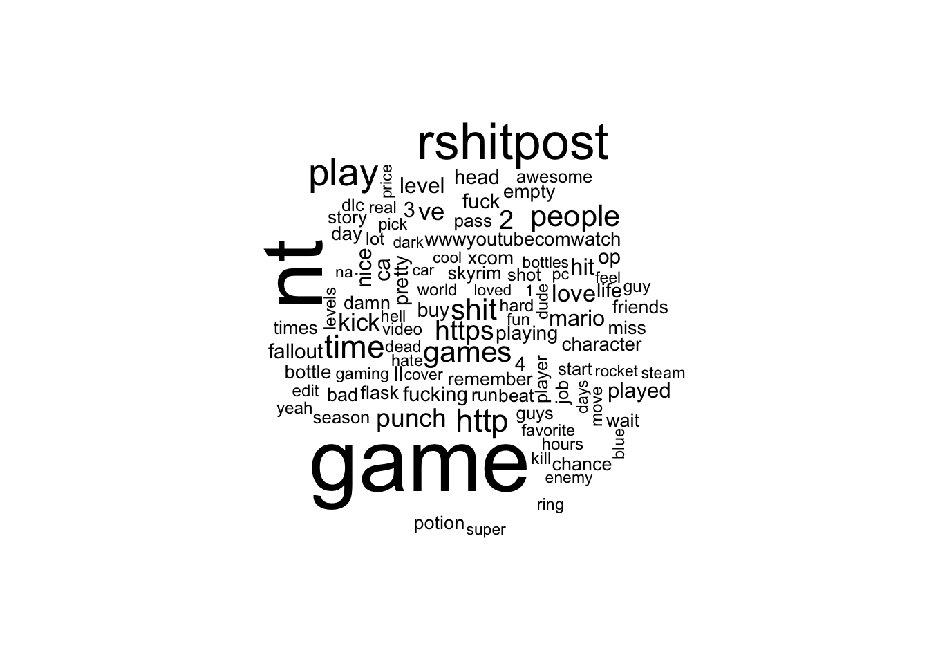
#We will come back to this, but this is coloring by sentiment
library('reshape2')
library('tidyr')

tidy_data %>%
  inner_join(get_sentiments('bing')) %>% #using the bing sentiment lexicon
  dplyr::count(word, sentiment, sort = TRUE) %>% #finding top words and pulling sentiment
  acast(word ~ sentiment, value.var = "n", fill = 0) %>%
  comparison.cloud(colors = c("#F8766D", "#00BFC4"), #adding color
                   max.words = 80) #max words to be plotted
## Joining, by = "word"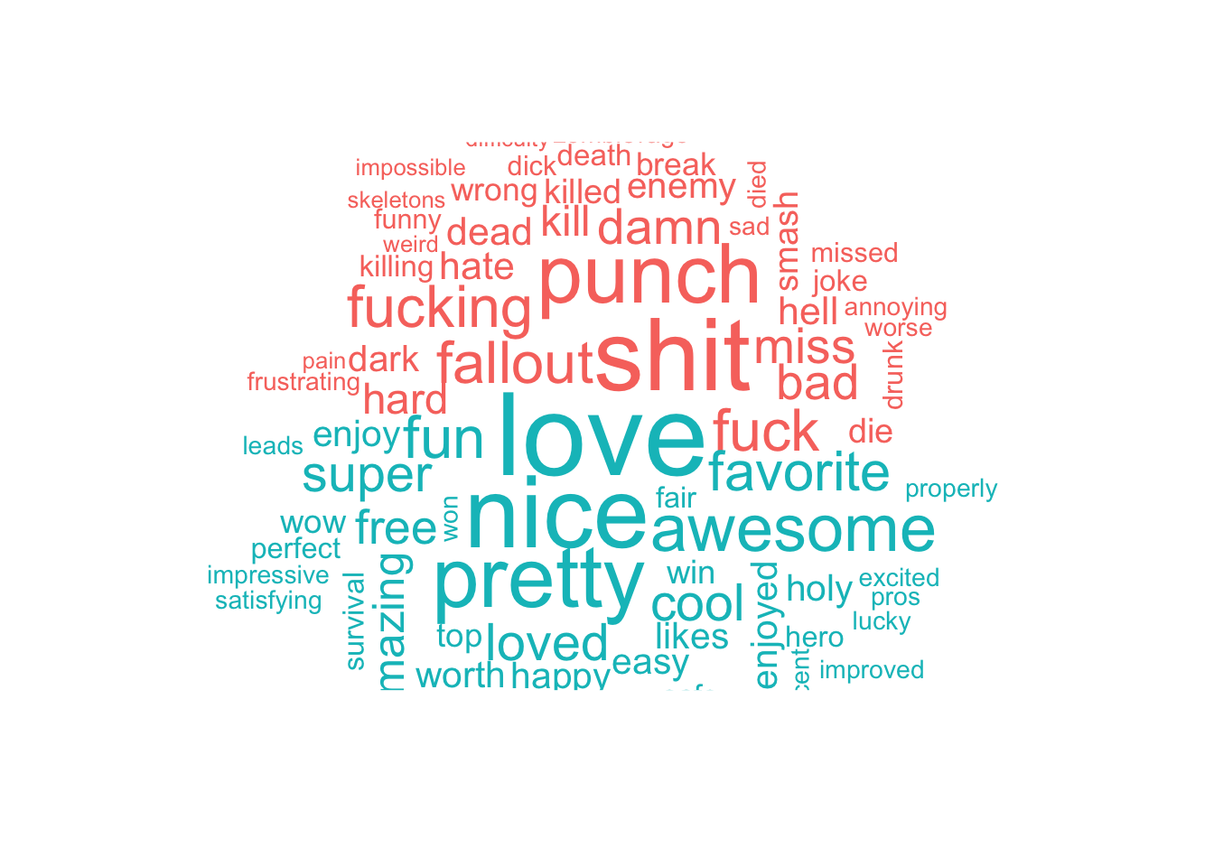
8.2 Lesson 2: Basic Sentiment Analysis
As we started to look at sentiment, above, it seems natural to continue looking at sentiment. Above, we looked at one of many sentiment lexicons, ‘bing’. Within the text mining packages we are using, there are 3 to choose from:
AFINN
bing
nrc
All three of these lexicons are based on unigrams, aka, single words. These lexicons contain many English words and the words are assigned scores for positive/negative sentiment, some have more categories such as joy, anger, sadness, etc. The nrc lexicon categorizes words in a binary fashion (“yes”/“no”) into categories of positive, negative, anger, anticipation, disgust, fear, joy, sadness, surprise, and trust. The bing lexicon categorizes words in a binary fashion into positive and negative categories. The AFINN lexicon assigns words with a score that runs between -5 and 5, with negative scores indicating negative sentiment and positive scores indicating positive sentiment.
We will focus on bing:
get_sentiments('bing')## # A tibble: 6,786 × 2
## word sentiment
## <chr> <chr>
## 1 2-faces negative
## 2 abnormal negative
## 3 abolish negative
## 4 abominable negative
## 5 abominably negative
## 6 abominate negative
## 7 abomination negative
## 8 abort negative
## 9 aborted negative
## 10 aborts negative
## # … with 6,776 more rows#here we are making a new dataframe pulling word, sentiment, and counts
bing_counts <- tidy_data %>%
inner_join(get_sentiments('bing')) %>%
dplyr::count(word, sentiment, sort = T)## Joining, by = "word"#we can visualize this like so:
bing_counts %>%
filter(n > 10) %>% #words have to occur more than 10 times
mutate(n = ifelse(sentiment == "negative", -n, n)) %>%
mutate(word = reorder(word, n)) %>% #ordring words
ggplot(aes(word, n, fill = sentiment)) + #plot
geom_col() +
coord_flip() +
labs(y = "Contribution to sentiment")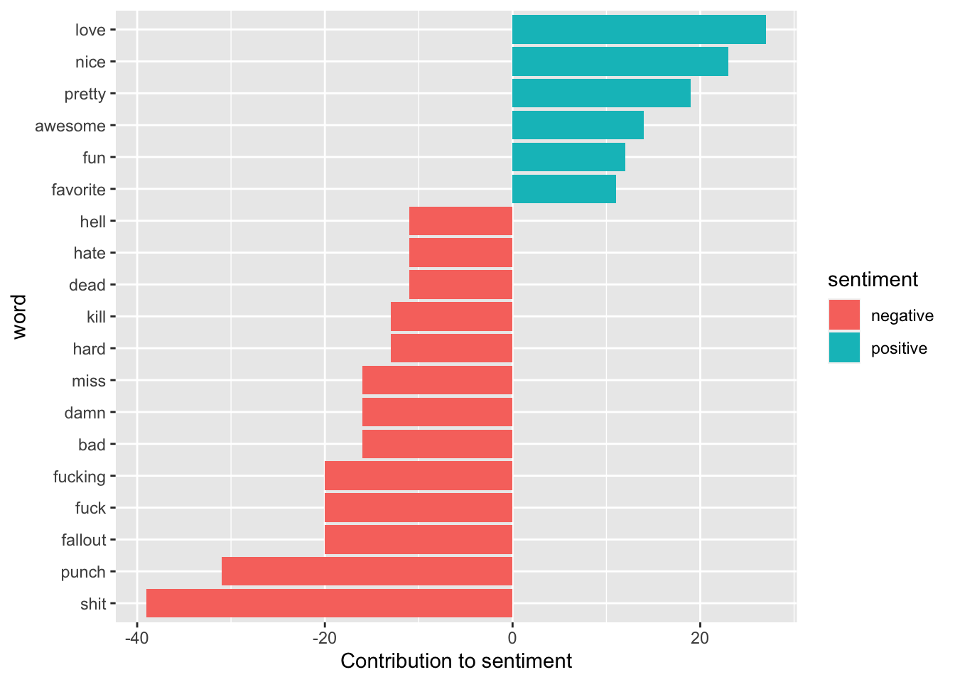 We can see that most of these words make sense for being positive or negative, however, depending on the context the word ‘miss’ could be a positive rather than negative. This is where knowing the data and the context in which these words are typically used is helpful. However, this also highlights the limitations of lexicon-based approaches where it is a unigram and takes the word at face value and does so without any context. If we needed to change and remove this word (or any other), we could easily add “miss” to a custom stop-words list using bind_rows().
8.2.1 Activity
Part 1: Discuss in 2-3 why this lexicon approach might be limited. Can you think of any examples where this could produce incorrect results? (hint: think of reviews)
Part 2: Using the text_OnlineMSc.csv file you’ve been given, which has data from 3 subreddits relating to news. Re-run all of the analysis above using this dataset.
What are the most common words in the news dataset overall?
What are the most common words in each of the subreddits?
What sentiment can we see in the dataset? Which words are the most sentient in the dataset? What about for each subreddit?
8.3 Lesson 3: Term-Frequency
TF-IDF is a measure that evaluates how relevant a word is to a document (and in a collection of documents). This is done by multiplying two metrics:
How many times a word appears in a document, and
Inverse document frequency of the word across a set of documents
TF or TF-IF has many uses, most importantly in automated text analysis, and can be useful for scoring words in machine learning algorithms for Natural Language Processing (NLP). TF-IDF (term frequency-inverse document frequency) was invented for document search and information retrieval because it works by increasing proportionally to the number of times a word appears in a document, but is offset by the number of documents that contain the word. Hence, words that are common in every document, such as this, what, and if, rank low even though they may appear many times, since they don’t mean much to that document. However, if the word ‘psychometric’ appears many times in a document, while not appearing many times in another document, it likely means that it’s relevant.
8.3.1 How are these calculated?
The term frequency of a word in a document can be calculated in a number of ways. The simplest is a raw count of instances a word appears in a document. This can then be adjusted by length of a document, or by the raw frequency of the most frequent word in a document.
The inverse document frequency of the word across a set of documents calculates how common or rare a word is in the entire document set. The closer it is to 0, the more common a word is. This metric can be calculated by taking the total number of documents, dividing it by the number of documents that contain a word, and calculating the logarithm.
- Therefore, if the word is very common and appears in many documents, this number will approach 0. Otherwise, it will approach 1.
8.3.2 Analyzing TF-IDF
The statistic tf-idf is intended to measure how important a word is to a document in a collection (or corpus) of documents, for example, to one novel in a collection of novels or to one website in a collection of websites.
Lets look at the text_OnlineMSC data.
## Warning: Missing column names filled in: 'X1' [1]## Warning: Duplicated column names deduplicated: 'X1' => 'X1_1' [2]##
## ── Column specification ──────────────────────────────────────────────────────────────────────────────────────────────────────────────────────────────────────────────
## cols(
## X1 = col_double(),
## X1_1 = col_double(),
## content = col_character(),
## subreddit = col_character()
## )library('dplyr')
sub_words <- news_sub %>%
unnest_tokens(word, content) %>%
dplyr::count(subreddit, word, sort = TRUE) #here we are getting counts of tokens
total_words <- sub_words %>%
group_by(subreddit) %>%
dplyr::summarise(total = sum(n))
head(total_words)## # A tibble: 3 × 2
## subreddit total
## <chr> <int>
## 1 news 230280
## 2 politics 12588
## 3 worldnews 15097sub_words <- dplyr::left_join(sub_words, total_words) #now joining these together## Joining, by = "subreddit"sub_words## # A tibble: 11,485 × 4
## subreddit word n total
## <chr> <chr> <int> <int>
## 1 news the 9834 230280
## 2 news to 6400 230280
## 3 news a 5181 230280
## 4 news and 4571 230280
## 5 news of 4344 230280
## 6 news i 3912 230280
## 7 news that 3436 230280
## 8 news it 3424 230280
## 9 news is 3196 230280
## 10 news in 3134 230280
## # … with 11,475 more rowsOf course, we can see here that n is the number of times the word has appeared in the document and as epxected, words like ‘the’ and ‘top’ are the top occurrences. There is a huge skew, where there are some words that appear incredibly often and then few words that are more unique. Lets have a look:
ggplot(sub_words, aes(n/total, fill = subreddit)) +
  geom_histogram(show.legend = FALSE) +
  xlim(NA, 0.0009) +
  facet_wrap(~subreddit, ncol = 2, scales = "free_y")
## `stat_bin()` using `bins = 30`. Pick better value with `binwidth`.## Warning: Removed 488 rows containing non-finite values (stat_bin).## Warning: Removed 3 rows containing missing values (geom_bar).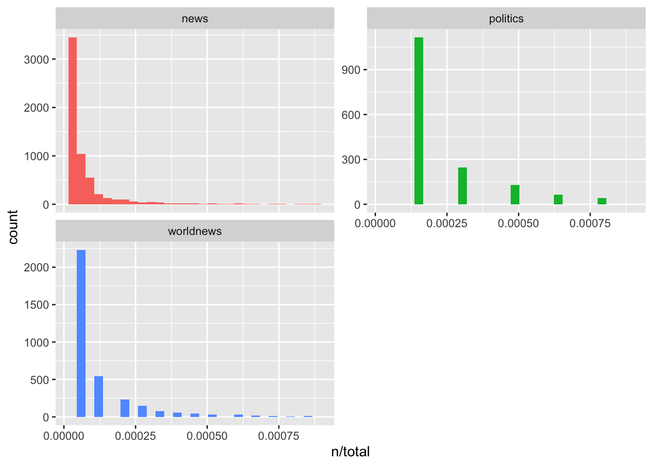
So, we can see long tails to the right for these novels (the more rare words!) that we have not shown in these plots. These plots exhibit similar distributions for all the novels, with many words that occur rarely and fewer words that occur frequently. This is absolutely normal and what you’d expect in anu corpus of natural language (e.g., books). This is called Zipf’s law, which states that the frequency that a word appears is inversely proportional to its rank.
Lets have a look at this:
freq_by_rank <- sub_words %>%
  group_by(subreddit) %>%
  dplyr::mutate(rank = row_number(),
         `term frequency` = n/total) %>%
  ungroup()

freq_by_rank
## # A tibble: 11,485 × 6
## subreddit word n total rank `term frequency`
## <chr> <chr> <int> <int> <int> <dbl>
## 1 news the 9834 230280 1 0.0427
## 2 news to 6400 230280 2 0.0278
## 3 news a 5181 230280 3 0.0225
## 4 news and 4571 230280 4 0.0198
## 5 news of 4344 230280 5 0.0189
## 6 news i 3912 230280 6 0.0170
## 7 news that 3436 230280 7 0.0149
## 8 news it 3424 230280 8 0.0149
## 9 news is 3196 230280 9 0.0139
## 10 news in 3134 230280 10 0.0136
## # … with 11,475 more rowsThe rank column here tells us the rank of each word within the frequency table; the table was already ordered by n so we could use row_number() to find the rank. Then, we can calculate the term frequency.
Zipf’s law is often visualized by plotting rank on the x-axis and term frequency on the y-axis, on logarithmic scales. Plotting this way, an inversely proportional relationship will have a constant, negative slope, like this:
freq_by_rank %>%
  ggplot(aes(rank, `term frequency`, color = subreddit)) +
  geom_line(size = 1.1, alpha = 0.8, show.legend = FALSE) +
  scale_x_log10() +
  scale_y_log10()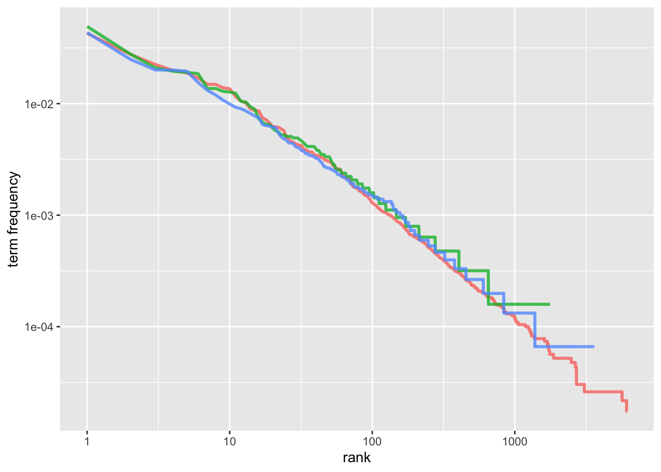
So, the lines are colored by subreddits, so we can see that all 3 subreddits are similar to one another, and the relationship between rank and frequency has a negative slope.
What next? Well, the idea of tf-idf is to find the most important words in a document, which happens by decreasing the weight for commonly used words (e.g., the) and increasing weight for words that are not used very much in a corpus (here, all three subreddits). To do this, we can use the bind_tf_idf() function in the tidytext package:
subs_tf_idf <- sub_words %>%
  bind_tf_idf(word, subreddit, n)

subs_tf_idf
## # A tibble: 11,485 × 7
## subreddit word n total tf idf tf_idf
## <chr> <chr> <int> <int> <dbl> <dbl> <dbl>
## 1 news the 9834 230280 0.0427 0 0
## 2 news to 6400 230280 0.0278 0 0
## 3 news a 5181 230280 0.0225 0 0
## 4 news and 4571 230280 0.0198 0 0
## 5 news of 4344 230280 0.0189 0 0
## 6 news i 3912 230280 0.0170 0 0
## 7 news that 3436 230280 0.0149 0 0
## 8 news it 3424 230280 0.0149 0 0
## 9 news is 3196 230280 0.0139 0 0
## 10 news in 3134 230280 0.0136 0 0
## # … with 11,475 more rowsNotice here the change between this output and the one the idf and thus tf-idf are zero for these extremely common words like the and to. These are all words that appear in all three subreddits, so the idf term (which will then be the natural log of 1) is zero.
The inverse document frequency (and thus tf-idf) is very low (near zero) for words that occur in many of the documents in a collection; this is how this approach decreases the weight for common words. The inverse document frequency will be a higher number for words that occur in fewer of the documents in the collection. So, lets look at the high tf-idfs…
subs_tf_idf %>%
  dplyr::select(-total) %>%
  arrange(desc(tf_idf))
## # A tibble: 11,485 × 6
## subreddit word n tf idf tf_idf
## <chr> <chr> <int> <dbl> <dbl> <dbl>
## 1 worldnews bot 40 0.00265 1.10 0.00291
## 2 worldnews quot 29 0.00192 1.10 0.00211
## 3 worldnews 039 26 0.00172 1.10 0.00189
## 4 worldnews turkey 25 0.00166 1.10 0.00182
## 5 politics bernie 52 0.00413 0.405 0.00167
## 6 worldnews 16 21 0.00139 1.10 0.00153
## 7 worldnews arabia 21 0.00139 1.10 0.00153
## 8 worldnews 23autotldr 20 0.00132 1.10 0.00146
## 9 worldnews constructive 20 0.00132 1.10 0.00146
## 10 worldnews drs 20 0.00132 1.10 0.00146
## # … with 11,475 more rowsHere, like with any text analytics, we need to consider how we cleaned the data – and this is an excellent example of messy data that will require additional removal of words in order to make sense of this. Hence, we might remove [[:digit:]] using regex methods to remove items like 039, which may have little meaning. Here, we would want to read some of the data and understand the context before we remove additional words.
However, let’s continue. We can visualize this, too:
library('forcats')

subs_tf_idf %>%
  group_by(subreddit) %>%
  slice_max(tf_idf, n = 15) %>%
  ungroup() %>%
  ggplot(aes(tf_idf, fct_reorder(word, tf_idf), fill = subreddit)) +
  geom_col(show.legend = FALSE) +
  facet_wrap(~subreddit, ncol = 2, scales = "free") +
  labs(x = "tf-idf", y = NULL)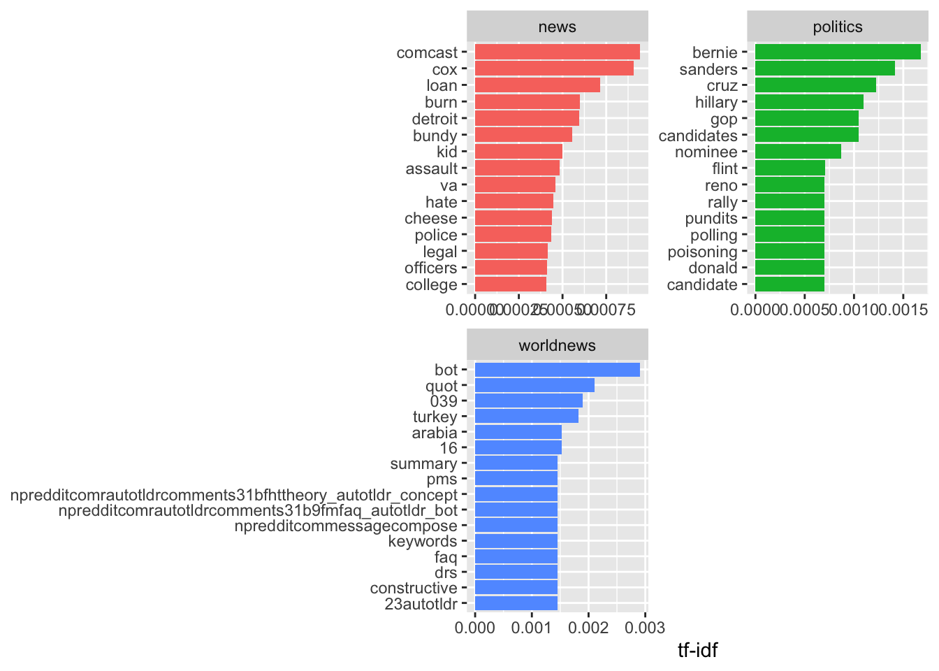
We can see there are some other data cleaning issues, where we can see long words chained together, which might be another subreddit or user that has been named. Hence, this process is incredibly iterative, and we might want to go back and filter out additional words, phrases, among other data artefacts. However, we can see some interesting terms appearing as highly important in these data, such as in r/politics, the term poisoning, donald (Trump), bernie, sanders, which demonstrates this is very US politics-oriented, whereas r/news is more focused on police, assult, and violence. Interestingly, r/worldnews is the least coherent, and requires additional data processing and cleaning to make sense of the outputs.