Chapter 4 Exploratory Data Analysis
In the next chapters, we will be looking at parts of exploratory data analysis (EDA). Here we will cover:
Looking at data
Basic Exploratory Data Analysis
Missing Data
Imputations (how to impute missing data)
Basic Overview of Statistics
4.1 Looking at data
Here, we will look primarily at the package dplyr (do have a look at the documentation), this is generally installed as part of the tidyverse package. dplyr is for data manipulation and is the newer person of plyr. We will look at some basic commands and things you’d generally want to have a look at when initially looking at data.
Lets have a look at iris:
library(tidyverse)
library(dplyr)

#you might wnt to look at the dimensions of a dataset, where we call dim()

dim(iris)
## [1] 150 5#we can just look at the dataset by calling it, here we can see iris is a 'tibble'
iris## Sepal.Length Sepal.Width Petal.Length Petal.Width Species
## 1 5.1 3.5 1.4 0.2 setosa
## 2 4.9 3.0 1.4 0.2 setosa
## 3 4.7 3.2 1.3 0.2 setosa
## 4 4.6 3.1 1.5 0.2 setosa
## 5 5.0 3.6 1.4 0.2 setosa
## 6 5.4 3.9 1.7 0.4 setosa
## 7 4.6 3.4 1.4 0.3 setosa
## 8 5.0 3.4 1.5 0.2 setosa
## 9 4.4 2.9 1.4 0.2 setosa
## 10 4.9 3.1 1.5 0.1 setosa
## 11 5.4 3.7 1.5 0.2 setosa
## 12 4.8 3.4 1.6 0.2 setosa
## 13 4.8 3.0 1.4 0.1 setosa
## 14 4.3 3.0 1.1 0.1 setosa
## 15 5.8 4.0 1.2 0.2 setosa
## 16 5.7 4.4 1.5 0.4 setosa
## 17 5.4 3.9 1.3 0.4 setosa
## 18 5.1 3.5 1.4 0.3 setosa
## 19 5.7 3.8 1.7 0.3 setosa
## 20 5.1 3.8 1.5 0.3 setosa
## 21 5.4 3.4 1.7 0.2 setosa
## 22 5.1 3.7 1.5 0.4 setosa
## 23 4.6 3.6 1.0 0.2 setosa
## 24 5.1 3.3 1.7 0.5 setosa
## 25 4.8 3.4 1.9 0.2 setosa
## 26 5.0 3.0 1.6 0.2 setosa
## 27 5.0 3.4 1.6 0.4 setosa
## 28 5.2 3.5 1.5 0.2 setosa
## 29 5.2 3.4 1.4 0.2 setosa
## 30 4.7 3.2 1.6 0.2 setosa
## 31 4.8 3.1 1.6 0.2 setosa
## 32 5.4 3.4 1.5 0.4 setosa
## 33 5.2 4.1 1.5 0.1 setosa
## 34 5.5 4.2 1.4 0.2 setosa
## 35 4.9 3.1 1.5 0.2 setosa
## 36 5.0 3.2 1.2 0.2 setosa
## 37 5.5 3.5 1.3 0.2 setosa
## 38 4.9 3.6 1.4 0.1 setosa
## 39 4.4 3.0 1.3 0.2 setosa
## 40 5.1 3.4 1.5 0.2 setosa
## 41 5.0 3.5 1.3 0.3 setosa
## 42 4.5 2.3 1.3 0.3 setosa
## 43 4.4 3.2 1.3 0.2 setosa
## 44 5.0 3.5 1.6 0.6 setosa
## 45 5.1 3.8 1.9 0.4 setosa
## 46 4.8 3.0 1.4 0.3 setosa
## 47 5.1 3.8 1.6 0.2 setosa
## 48 4.6 3.2 1.4 0.2 setosa
## 49 5.3 3.7 1.5 0.2 setosa
## 50 5.0 3.3 1.4 0.2 setosa
## 51 7.0 3.2 4.7 1.4 versicolor
## 52 6.4 3.2 4.5 1.5 versicolor
## 53 6.9 3.1 4.9 1.5 versicolor
## 54 5.5 2.3 4.0 1.3 versicolor
## 55 6.5 2.8 4.6 1.5 versicolor
## 56 5.7 2.8 4.5 1.3 versicolor
## 57 6.3 3.3 4.7 1.6 versicolor
## 58 4.9 2.4 3.3 1.0 versicolor
## 59 6.6 2.9 4.6 1.3 versicolor
## 60 5.2 2.7 3.9 1.4 versicolor
## 61 5.0 2.0 3.5 1.0 versicolor
## 62 5.9 3.0 4.2 1.5 versicolor
## 63 6.0 2.2 4.0 1.0 versicolor
## 64 6.1 2.9 4.7 1.4 versicolor
## 65 5.6 2.9 3.6 1.3 versicolor
## 66 6.7 3.1 4.4 1.4 versicolor
## 67 5.6 3.0 4.5 1.5 versicolor
## 68 5.8 2.7 4.1 1.0 versicolor
## 69 6.2 2.2 4.5 1.5 versicolor
## 70 5.6 2.5 3.9 1.1 versicolor
## 71 5.9 3.2 4.8 1.8 versicolor
## 72 6.1 2.8 4.0 1.3 versicolor
## 73 6.3 2.5 4.9 1.5 versicolor
## 74 6.1 2.8 4.7 1.2 versicolor
## 75 6.4 2.9 4.3 1.3 versicolor
## 76 6.6 3.0 4.4 1.4 versicolor
## 77 6.8 2.8 4.8 1.4 versicolor
## 78 6.7 3.0 5.0 1.7 versicolor
## 79 6.0 2.9 4.5 1.5 versicolor
## 80 5.7 2.6 3.5 1.0 versicolor
## 81 5.5 2.4 3.8 1.1 versicolor
## 82 5.5 2.4 3.7 1.0 versicolor
## 83 5.8 2.7 3.9 1.2 versicolor
## 84 6.0 2.7 5.1 1.6 versicolor
## 85 5.4 3.0 4.5 1.5 versicolor
## 86 6.0 3.4 4.5 1.6 versicolor
## 87 6.7 3.1 4.7 1.5 versicolor
## 88 6.3 2.3 4.4 1.3 versicolor
## 89 5.6 3.0 4.1 1.3 versicolor
## 90 5.5 2.5 4.0 1.3 versicolor
## 91 5.5 2.6 4.4 1.2 versicolor
## 92 6.1 3.0 4.6 1.4 versicolor
## 93 5.8 2.6 4.0 1.2 versicolor
## 94 5.0 2.3 3.3 1.0 versicolor
## 95 5.6 2.7 4.2 1.3 versicolor
## 96 5.7 3.0 4.2 1.2 versicolor
## 97 5.7 2.9 4.2 1.3 versicolor
## 98 6.2 2.9 4.3 1.3 versicolor
## 99 5.1 2.5 3.0 1.1 versicolor
## 100 5.7 2.8 4.1 1.3 versicolor
## 101 6.3 3.3 6.0 2.5 virginica
## 102 5.8 2.7 5.1 1.9 virginica
## 103 7.1 3.0 5.9 2.1 virginica
## 104 6.3 2.9 5.6 1.8 virginica
## 105 6.5 3.0 5.8 2.2 virginica
## 106 7.6 3.0 6.6 2.1 virginica
## 107 4.9 2.5 4.5 1.7 virginica
## 108 7.3 2.9 6.3 1.8 virginica
## 109 6.7 2.5 5.8 1.8 virginica
## 110 7.2 3.6 6.1 2.5 virginica
## 111 6.5 3.2 5.1 2.0 virginica
## 112 6.4 2.7 5.3 1.9 virginica
## 113 6.8 3.0 5.5 2.1 virginica
## 114 5.7 2.5 5.0 2.0 virginica
## 115 5.8 2.8 5.1 2.4 virginica
## 116 6.4 3.2 5.3 2.3 virginica
## 117 6.5 3.0 5.5 1.8 virginica
## 118 7.7 3.8 6.7 2.2 virginica
## 119 7.7 2.6 6.9 2.3 virginica
## 120 6.0 2.2 5.0 1.5 virginica
## 121 6.9 3.2 5.7 2.3 virginica
## 122 5.6 2.8 4.9 2.0 virginica
## 123 7.7 2.8 6.7 2.0 virginica
## 124 6.3 2.7 4.9 1.8 virginica
## 125 6.7 3.3 5.7 2.1 virginica
## 126 7.2 3.2 6.0 1.8 virginica
## 127 6.2 2.8 4.8 1.8 virginica
## 128 6.1 3.0 4.9 1.8 virginica
## 129 6.4 2.8 5.6 2.1 virginica
## 130 7.2 3.0 5.8 1.6 virginica
## 131 7.4 2.8 6.1 1.9 virginica
## 132 7.9 3.8 6.4 2.0 virginica
## 133 6.4 2.8 5.6 2.2 virginica
## 134 6.3 2.8 5.1 1.5 virginica
## 135 6.1 2.6 5.6 1.4 virginica
## 136 7.7 3.0 6.1 2.3 virginica
## 137 6.3 3.4 5.6 2.4 virginica
## 138 6.4 3.1 5.5 1.8 virginica
## 139 6.0 3.0 4.8 1.8 virginica
## 140 6.9 3.1 5.4 2.1 virginica
## 141 6.7 3.1 5.6 2.4 virginica
## 142 6.9 3.1 5.1 2.3 virginica
## 143 5.8 2.7 5.1 1.9 virginica
## 144 6.8 3.2 5.9 2.3 virginica
## 145 6.7 3.3 5.7 2.5 virginica
## 146 6.7 3.0 5.2 2.3 virginica
## 147 6.3 2.5 5.0 1.9 virginica
## 148 6.5 3.0 5.2 2.0 virginica
## 149 6.2 3.4 5.4 2.3 virginica
## 150 5.9 3.0 5.1 1.8 virginica#then we might want to look at the first 10 rows of the dataset
head(iris, 10) #number at the end states number of rows## Sepal.Length Sepal.Width Petal.Length Petal.Width Species
## 1 5.1 3.5 1.4 0.2 setosa
## 2 4.9 3.0 1.4 0.2 setosa
## 3 4.7 3.2 1.3 0.2 setosa
## 4 4.6 3.1 1.5 0.2 setosa
## 5 5.0 3.6 1.4 0.2 setosa
## 6 5.4 3.9 1.7 0.4 setosa
## 7 4.6 3.4 1.4 0.3 setosa
## 8 5.0 3.4 1.5 0.2 setosa
## 9 4.4 2.9 1.4 0.2 setosa
## 10 4.9 3.1 1.5 0.1 setosaHere, it is important to note that this is not just a data.frame (a typical format we see in base R), but this is a dataset is in the form of a tibble, which is a data.frame in the tidyverse. You can see this in the console when you run certain code. This is a ‘modern reimagining of the data.frame’, which you can read about here (https://tibble.tidyverse.org/), however, they are useful for handling larger datasets with complex objects within it. However, this is just something to keep an eye on, as this format is not always cross-compatible with other packages that might need a data.frame.
When first looking at data, there are a number of commands we can look at using dplyr, which will help your EDA. We can focus on commands that impacts the:
- Rows
filter()- takes rows based on column values (e.g., for numeric rows, you can filter on value using >, <, etc., or filter on categorical values using == ’’)arrange()- changes the order of rows (e.g., change to ascending or descending order, this can be useful when doing data viz)
- Columns
select()- literally selects columns to be included (e.g., you are creating a new data.frame/tibble with only certain columns)rename()- if you want to rename columns for ease of plotting/analysismutate()- creates a new column/variable and preserves the datasettransmute()- use with caution, this adds new variables and drops existing ones
- Groups
summarise()- this collapses or aggregates data into a single row (e.g., by the mean, median), this can also be mixed with group_by() in order to summarise by groups (e.g., male, female or other categorical variables)
…Please note, this is not exhaustive of the functions in dplyr, please look at the documentation. These are ones I’ve pulled as perhaps the most useful and common you’ll see and likely need when doing general data cleaning, processing, and analyses.
Another key feature of dplyr that will come in useful is the ability to ‘pipe’, which is the %>% operator. I think the easiest way to think of %>% is AND THEN do a thing. So see the example below, this literally means, take the iris dataset, AND THEN filter it (whereby only pull through observations that are setosa). Note here, we are not creating a new dataframe, so this will just print in the console.
iris %>% filter(Species == 'setosa') #so you can see that the dataset printed now only consists of setosa rows## Sepal.Length Sepal.Width Petal.Length Petal.Width Species
## 1 5.1 3.5 1.4 0.2 setosa
## 2 4.9 3.0 1.4 0.2 setosa
## 3 4.7 3.2 1.3 0.2 setosa
## 4 4.6 3.1 1.5 0.2 setosa
## 5 5.0 3.6 1.4 0.2 setosa
## 6 5.4 3.9 1.7 0.4 setosa
## 7 4.6 3.4 1.4 0.3 setosa
## 8 5.0 3.4 1.5 0.2 setosa
## 9 4.4 2.9 1.4 0.2 setosa
## 10 4.9 3.1 1.5 0.1 setosa
## 11 5.4 3.7 1.5 0.2 setosa
## 12 4.8 3.4 1.6 0.2 setosa
## 13 4.8 3.0 1.4 0.1 setosa
## 14 4.3 3.0 1.1 0.1 setosa
## 15 5.8 4.0 1.2 0.2 setosa
## 16 5.7 4.4 1.5 0.4 setosa
## 17 5.4 3.9 1.3 0.4 setosa
## 18 5.1 3.5 1.4 0.3 setosa
## 19 5.7 3.8 1.7 0.3 setosa
## 20 5.1 3.8 1.5 0.3 setosa
## 21 5.4 3.4 1.7 0.2 setosa
## 22 5.1 3.7 1.5 0.4 setosa
## 23 4.6 3.6 1.0 0.2 setosa
## 24 5.1 3.3 1.7 0.5 setosa
## 25 4.8 3.4 1.9 0.2 setosa
## 26 5.0 3.0 1.6 0.2 setosa
## 27 5.0 3.4 1.6 0.4 setosa
## 28 5.2 3.5 1.5 0.2 setosa
## 29 5.2 3.4 1.4 0.2 setosa
## 30 4.7 3.2 1.6 0.2 setosa
## 31 4.8 3.1 1.6 0.2 setosa
## 32 5.4 3.4 1.5 0.4 setosa
## 33 5.2 4.1 1.5 0.1 setosa
## 34 5.5 4.2 1.4 0.2 setosa
## 35 4.9 3.1 1.5 0.2 setosa
## 36 5.0 3.2 1.2 0.2 setosa
## 37 5.5 3.5 1.3 0.2 setosa
## 38 4.9 3.6 1.4 0.1 setosa
## 39 4.4 3.0 1.3 0.2 setosa
## 40 5.1 3.4 1.5 0.2 setosa
## 41 5.0 3.5 1.3 0.3 setosa
## 42 4.5 2.3 1.3 0.3 setosa
## 43 4.4 3.2 1.3 0.2 setosa
## 44 5.0 3.5 1.6 0.6 setosa
## 45 5.1 3.8 1.9 0.4 setosa
## 46 4.8 3.0 1.4 0.3 setosa
## 47 5.1 3.8 1.6 0.2 setosa
## 48 4.6 3.2 1.4 0.2 setosa
## 49 5.3 3.7 1.5 0.2 setosa
## 50 5.0 3.3 1.4 0.2 setosaTo use this as a new dataset, you can create it (using assignment operators, I tend to use ‘=’ however is it common in R to use ‘<-’). Creating a new dataset to be used in the R environment, we give it a name: iris_setosa, and then assign something to it. These can be dataframes (or tibbles in this case) or they can be a list, vector, among other formats. It is useful to know about these structures for more advanced programming.
iris_setosa = iris %>%
  filter(Species == 'setosa')

head(iris_setosa)
## Sepal.Length Sepal.Width Petal.Length Petal.Width Species
## 1 5.1 3.5 1.4 0.2 setosa
## 2 4.9 3.0 1.4 0.2 setosa
## 3 4.7 3.2 1.3 0.2 setosa
## 4 4.6 3.1 1.5 0.2 setosa
## 5 5.0 3.6 1.4 0.2 setosa
## 6 5.4 3.9 1.7 0.4 setosa#we can check that this has filtered out any other species using unique()
unique(iris_setosa$Species)## [1] setosa
## Levels: setosa versicolor virginica#this shows only one level (aka only setosa) as this is a factor variableIf you want to select columns, lets try it using the diamonds dataset as an example and select particular columns:
head(diamonds) ## # A tibble: 6 × 10
## carat cut color clarity depth table price x y z
## <dbl> <ord> <ord> <ord> <dbl> <dbl> <int> <dbl> <dbl> <dbl>
## 1 0.23 Ideal E SI2 61.5 55 326 3.95 3.98 2.43
## 2 0.21 Premium E SI1 59.8 61 326 3.89 3.84 2.31
## 3 0.23 Good E VS1 56.9 65 327 4.05 4.07 2.31
## 4 0.29 Premium I VS2 62.4 58 334 4.2 4.23 2.63
## 5 0.31 Good J SI2 63.3 58 335 4.34 4.35 2.75
## 6 0.24 Very Good J VVS2 62.8 57 336 3.94 3.96 2.48#lets select carat, cut, color, and clarity only
#here we are creating a new dataframe called smaller_diamonds, then we call the SELECT command
#and then list the variables we want to keep
smaller_diamonds = dplyr::select(diamonds,
carat,
cut,
color,
clarity)
head(smaller_diamonds)## # A tibble: 6 × 4
## carat cut color clarity
## <dbl> <ord> <ord> <ord>
## 1 0.23 Ideal E SI2
## 2 0.21 Premium E SI1
## 3 0.23 Good E VS1
## 4 0.29 Premium I VS2
## 5 0.31 Good J SI2
## 6 0.24 Very Good J VVS2You can use additional functions with select, such as:
* starts_with() - where you define a start pattern that is selected (e.g., ‘c’ in the diamonds package should pull all columns starting with ‘c’)
* ends_with() - pulls anything that ends with a defined pattern
* matches() - matches a specific regular expression (to be explained later)
* contains() - contains a literal string (e.g., ‘ri’ will only bring through pRIce and claRIty)
(Examples to be added…)
If you ever find you want to rename variables for any reason… do it sooner rather than later. Also, sometimes it is easier to do this outside of R… however, this is how to do this:
#lets rename the price variable as price tag
#again we are creating a new dataset
#THEN %>% we are calling rename() and then renaming by defining the new name = old name
diamond_rename = diamonds %>%
  dplyr::rename(price_tag = price)

head(diamond_rename) #check
## # A tibble: 6 × 10
## carat cut color clarity depth table price_tag x y z
## <dbl> <ord> <ord> <ord> <dbl> <dbl> <int> <dbl> <dbl> <dbl>
## 1 0.23 Ideal E SI2 61.5 55 326 3.95 3.98 2.43
## 2 0.21 Premium E SI1 59.8 61 326 3.89 3.84 2.31
## 3 0.23 Good E VS1 56.9 65 327 4.05 4.07 2.31
## 4 0.29 Premium I VS2 62.4 58 334 4.2 4.23 2.63
## 5 0.31 Good J SI2 63.3 58 335 4.34 4.35 2.75
## 6 0.24 Very Good J VVS2 62.8 57 336 3.94 3.96 2.48So, lets create some new variables! Here, we use the mutate() function. Lets fiddle around with the diamonds dataset:
# Lets change the price by halving it...
# we will reuse the diamond_rename as we'll use the original diamonds one later

diamond_rename %>%
  dplyr::mutate(half_price = price_tag/2)
## # A tibble: 53,940 × 11
## carat cut color clarity depth table price_tag x y z half_price
## <dbl> <ord> <ord> <ord> <dbl> <dbl> <int> <dbl> <dbl> <dbl> <dbl>
## 1 0.23 Ideal E SI2 61.5 55 326 3.95 3.98 2.43 163
## 2 0.21 Premium E SI1 59.8 61 326 3.89 3.84 2.31 163
## 3 0.23 Good E VS1 56.9 65 327 4.05 4.07 2.31 164.
## 4 0.29 Premium I VS2 62.4 58 334 4.2 4.23 2.63 167
## 5 0.31 Good J SI2 63.3 58 335 4.34 4.35 2.75 168.
## 6 0.24 Very Good J VVS2 62.8 57 336 3.94 3.96 2.48 168
## 7 0.24 Very Good I VVS1 62.3 57 336 3.95 3.98 2.47 168
## 8 0.26 Very Good H SI1 61.9 55 337 4.07 4.11 2.53 168.
## 9 0.22 Fair E VS2 65.1 61 337 3.87 3.78 2.49 168.
## 10 0.23 Very Good H VS1 59.4 61 338 4 4.05 2.39 169
## # … with 53,930 more rows# we can create multiple new columns at once
diamond_rename %>%
dplyr::mutate(price300 = price_tag - 300, # 300 OFF from the original price
price30perc = price_tag * 0.30, # 30% of the original price
price30percoff = price_tag * 0.70, # 30% OFF from the original price
pricepercarat = price_tag / carat) # ratio of price to carat## # A tibble: 53,940 × 14
## carat cut color clarity depth table price_tag x y z price300 price30perc price30percoff pricepercarat
## <dbl> <ord> <ord> <ord> <dbl> <dbl> <int> <dbl> <dbl> <dbl> <dbl> <dbl> <dbl> <dbl>
## 1 0.23 Ideal E SI2 61.5 55 326 3.95 3.98 2.43 26 97.8 228. 1417.
## 2 0.21 Premium E SI1 59.8 61 326 3.89 3.84 2.31 26 97.8 228. 1552.
## 3 0.23 Good E VS1 56.9 65 327 4.05 4.07 2.31 27 98.1 229. 1422.
## 4 0.29 Premium I VS2 62.4 58 334 4.2 4.23 2.63 34 100. 234. 1152.
## 5 0.31 Good J SI2 63.3 58 335 4.34 4.35 2.75 35 100. 234. 1081.
## 6 0.24 Very Good J VVS2 62.8 57 336 3.94 3.96 2.48 36 101. 235. 1400
## 7 0.24 Very Good I VVS1 62.3 57 336 3.95 3.98 2.47 36 101. 235. 1400
## 8 0.26 Very Good H SI1 61.9 55 337 4.07 4.11 2.53 37 101. 236. 1296.
## 9 0.22 Fair E VS2 65.1 61 337 3.87 3.78 2.49 37 101. 236. 1532.
## 10 0.23 Very Good H VS1 59.4 61 338 4 4.05 2.39 38 101. 237. 1470.
## # … with 53,930 more rows4.2 Basic EDA
EDA is an iterative cycle. What we looked at above is definitely part of EDA, but it was also to give a little overview of the dplyr package and some of the main commands that will likely be useful if you are newer to R. However, there are a number of tutorials out there that will teach you more about R programming.
Let’s look at EDA more closely. What is it and what will you be doing?
Generating questions about your data,
Search for answers by visualising, transforming, and modelling your data, and
Use what you learn to refine your questions and/or generate new questions.
We will cover all of this over the next two chapters EDA is not a formal process with a strict set of rules. More than anything, EDA is the analyst’s time to actually get to know your data and understand what you can really do with it. During the initial phases of EDA you should feel free to investigate every idea that occurs to you. This is all about understanding your data. Some of these ideas will pan out, and some will be dead ends. All of it is important and will help you figure out your questions… additionally, this is important to log and do not worry about ‘null’ findings, these are just as important!
It is important to point out here that this will get easier and better with practice and experience. The more you look at data and the more time you work with it, the easier you’ll find it to spot odd artefacts in there. For instance, I’ve looked at haul truck data recently (don’t ask…) and to give you an idea of what I am talking about: these are three-storey high trucks and weigh about 300-tonnes – now, the data said one of these moved at >1,000km/hr… Hopefully, this is absolutely not true as this is horrifuing, but also hopefully you’ve also realized this is also very unlikely. In other data coming from smartphones, in the EDA process, we found various have missing data – where it is difficult to know whether this was a logging error or something else. However, the interesting and important discussion is to (a) find out why this may have happened, (b) what does this mean for the data, (c) what do we do with this missing data, (d) is this a one-off or has this happened elsewhere too, and (e) what does this mean for the participants involved in terms of what inferences we will draw on our findings?
4.2.1 Brief ethics consideration based on point (e)
When thinking about data, often (not always) this comes from people. One thing I want to stress in this work, despite at present, this uses non-human data in the first chapters (to be updated), remember you are handling people’s data. Each observation (usually) is a person, and if you were that person, how would you feel about how you are using these data? Are you making fair judgement and assessments? How are you justifying your decision making? If there are ‘outliers’ – who are they? Was this a genuine data entry/logging error or was this real data, are you discriminating against a sub-set of the population by removing them? It is critically important to consider the consequences of every decision you make when doing data analysis. Unfortunately there is no tool or framework for this, this is down to you for the most part, and for you to be open, honest, and think about what you’re doing…
(to be expanded and have another chapter on this…)
4.2.2 Quick reminders of definitions for EDA
A variable is a quantity, quality, or property that you can measure.
A value is the state of a variable when you measure it. The value of a variable may change from measurement to measurement.
An observation is a set of measurements made under similar conditions (you usually make all of the measurements in an observation at the same time and on the same object). An observation will contain several values, each associated with a different variable. I’ll sometimes refer to an observation as a data point.
Tabular data is a set of values, each associated with a variable and an observation. Tabular data is tidy if each value is placed in its own “cell”, each variable in its own column, and each observation in its own row.
4.2.3 Variation
Variation is the tendency of the values of a variable to change from measurement to measurement. You can see variation easily in real life; if you measure any continuous variable twice, you will get two different results. This is true even if you measure quantities that are constant, like the speed of light. Each of your measurements will include a small amount of error that varies from measurement to measurement.
(This is why in STEM fields, equipment needs to be calibrated before use… this is not a thing in the social sciences, which is an interesting issue in itself – to be expanded upon in another forthcoming chapter).
Categorical variables can also vary if you measure across different subjects (e.g., the eye colors of different people), or different times (e.g. the energy levels of an electron at different moments). Every variable has its own pattern of variation, which can reveal interesting information. The best way to understand that pattern is to visualize the distribution of the variable’s values. It is important to understand the variation in your datasets, and one of the easiest ways to look at this is to visualize it (we will have a chapter purely on data visualization, too). Let’s start with loading in the following libraries (or installing them using the command install.packages() making sure to use quote around each package called): dplyr, tidyverse, magrittr, and ggplot2.
How you visualise the distribution of a variable will depend on whether the variable is categorical or continuous. A variable is categorical if it can only take one of a small set of values (e.g., color, size, level of education). These can also be ranked or ordered. In R, categorical variables are usually saved as factors or character vectors. To examine the distribution of a categorical variable, use a bar chart:
library('dplyr')
library('magrittr')
library('ggplot2')
library('tidyverse')

#Here we will look at the diamonds dataset
#lets look at the variable cut, which is a categorical variable, but how do you check?
#ypu can check using the is.factor() command and it'll return a boolean TRUE or FALSE
is.factor(diamonds$cut) #here we call the diamonds dataset and use the $ sign to specify which column
## [1] TRUE#if something is not a factor when it needs to be, you can use the
# as.factor() command, but check using is.factor() after to ensure this worked as anticipated
#lets have a visualize the diamonds dataset using a bar plot
ggplot(data = diamonds) +
geom_bar(mapping = aes(x = cut))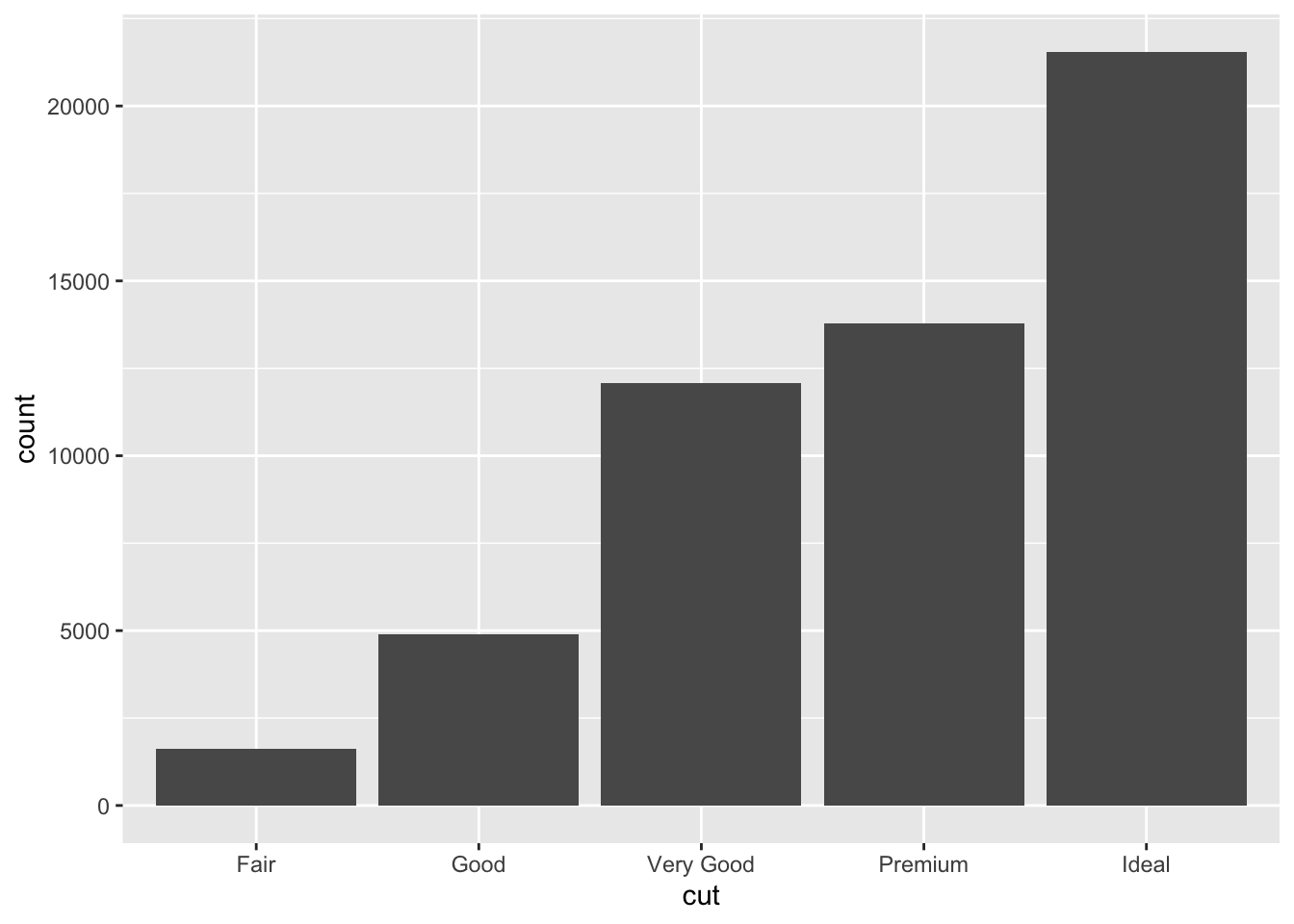
You can also look at this without data visualization, for example using the count command in dplyr.
#this will give you a count per each category. There are a number of ways to do this, but this is the most simple:
#note we are calling dplyr:: here as this count command can be masked by other packages, this is just to ensure this code runs
diamonds %>%
  dplyr::count(cut)
## # A tibble: 5 × 2
## cut n
## <ord> <int>
## 1 Fair 1610
## 2 Good 4906
## 3 Very Good 12082
## 4 Premium 13791
## 5 Ideal 21551If we are looking at continuous variables, a histogram is the better way to look at the distribution of each variable:
ggplot(data = diamonds) +
  geom_histogram(mapping = aes(x = carat), binwidth = 0.5)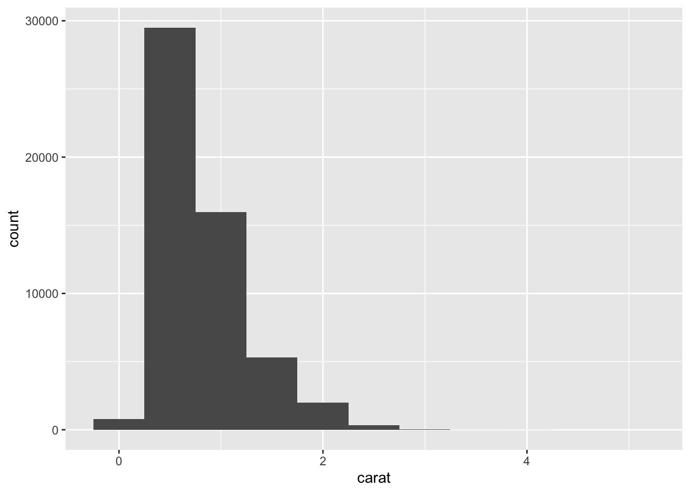
A histogram divides the x-axis into equally spaced bins and then uses the height of a bar to display the number of observations that fall in each bin. In the graph above, the tallest bar shows that almost 30,000 observations have a carat value between 0.25 and 0.75, which are the left and right edges of the bar.
You can set the width of the intervals in a histogram with the binwidth argument, which is measured in the units of the x variable. You should always explore a variety of binwidths when working with histograms, as different binwidths can reveal different patterns. It is really important to experiemnt and get this right otherwise you’ll see too much or too little variation in the variable. Please note: you should do this for every variable you have so you can understand how much or little variation you have in your daatset and whether it is normally distributed or not (e.g., the histogram looks like a bell curve).
For example, here is how the graph above looks when we zoom into just the diamonds with a size of less than three carats and choose a smaller binwidth:
smaller <- diamonds %>%
  filter(carat < 3)

ggplot(data = smaller, mapping = aes(x = carat)) +
  geom_histogram(binwidth = 0.01)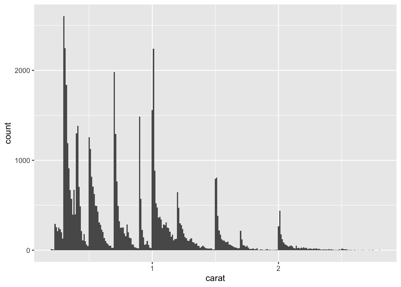
So, if we look at the classic iris dataset, what naturally occurring groups can we see? In the code below, you can see that there are two key groups here, petals that are quite small (<2cm) and larger petals (>3cm).
ggplot(data = iris, mapping = aes(x = Petal.Length)) +
  geom_histogram(binwidth = 0.25)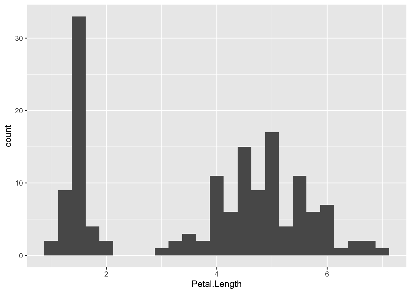
Another example is in the eruptions of the Old Faithful Geyser in Yellowstone National Park dataset. Eruption times appear to be clustered into two groups: there are short eruptions (of around 2 minutes) and long eruptions (4-5 minutes), but little in between.
ggplot(data = faithful, mapping = aes(x = eruptions)) +
  geom_histogram(binwidth = 0.25)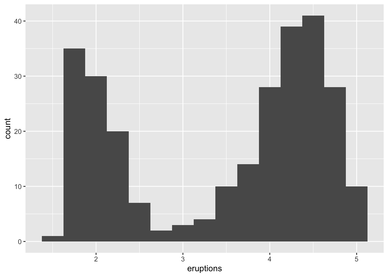
4.2.4 Data in Context, part 2
When you look at your data, you might find some outliers, or extreme values that are unusual or unexpected. These are extremely important to address and investigate as these might be data entry issues (e.g., with technology usage time estimates, when asked how long do you use your phone each day (hours) and someone inputs 23 (hours) might be a mistake, this could be a sensor logging issue) or this may be an interesting artifact in your dataset.
It is important here to understand what are expected and unexpected values. When you’re working in a new context it is critical for you to ask data owners, or whomever collected it, or someone who knows the context for help. Do not come up with your own rules on this because you do not have enough knowledge. Be risk adverse, it is better to be a little slower and get things right than to rush and potentially cause some issues down the line, as mistakes here will only get bigger as these data are further analysed. It is common to see rules of thumb that mean anything +/- 3SDs should be removed from analyses. This is not always a good idea without knowing the context and whether this is actually appropriate.
4.2.5 Ethics interjection
As we talked about a little before – what if those ‘extreme’ values are genuine? What if these are typically underrepresented sub-groups of a population and we are now just removing them without reason? It is important to think carefully about your RQs and consider what you are doing before just removing data with a simple rule of thumb. If these are underrepresented groups being removed, this may end up continuing to solidify a bias seen in data so be careful.
So, if we look again at the diamonds dataset, specifically looking at the distribution of the variable ‘y’, which is the ‘width in mm’ of each diamond, we get the following histogram:
ggplot(diamonds) +
geom_histogram(mapping = aes(x = y), binwidth = 0.5)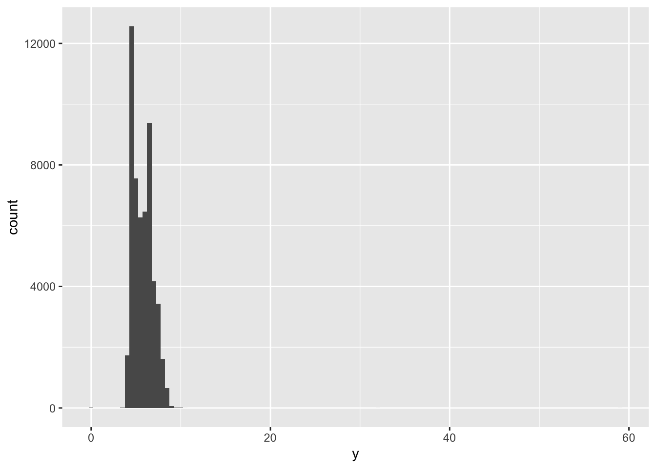 This clearly shows there is something extreme happening, (also noting these data are about diamonds not people so we can tailor our thinking accordingly)… here we can see this a rare occurrence as we can hardly see the bars towards the right-hand side of the plot.
Let’s look at this more…
# note be careful with code command duplicate names... if your code worked once and errors another time, it might be due to conflicts
#hence here, we call select using dpylr:: to ensure this does not happen
unusual <- diamonds %>%
  filter(y < 3 | y > 20) %>%
  dplyr::select(price, x, y, z) %>%
  arrange(y)
unusual
## # A tibble: 9 × 4
## price x y z
## <int> <dbl> <dbl> <dbl>
## 1 5139 0 0 0
## 2 6381 0 0 0
## 3 12800 0 0 0
## 4 15686 0 0 0
## 5 18034 0 0 0
## 6 2130 0 0 0
## 7 2130 0 0 0
## 8 2075 5.15 31.8 5.12
## 9 12210 8.09 58.9 8.06The y variable (width in mm) measures one of the three dimensions of these diamonds (all in mm)… so what do we infer here? Well, we know that diamonds can’t have a width of 0mm, so these values must be incorrect. Similarly, at the other extreme, we might also suspect that measurements of 32mm and 59mm are implausible: those diamonds are over an inch long, but don’t cost hundreds of thousands of dollars! (this is why it is important to look at distributions in context of other variables, like price!)
It’s good practice to repeat your analysis with and without the outliers. If they have minimal effect on the results, and you can’t figure out why they’re there, it’s reasonable to drop them move on (but keep note of the number of observations you remove and why). However, if they have a substantial effect on your results, you shouldn’t drop them without justification. There may be reasons, for example, completely implausible observations (e.g., someone reporting they use their smartphone for more than 24 hours in a day), but others may be worth further investigation and decision-making. You’ll need to figure out what caused them (e.g. a data entry error) and disclose that you removed them (or not) in write ups.
4.2.6 Covariation
If variation describes the behavior within a variable, covariation describes the behavior between variables. Covariation is the tendency for the values of two or more variables to vary together in a related way. The best way to spot covariation is to visualize the relationship between two or more variables.
4.2.6.1 Categorical and Continuous Variables
Let’s look back at the diamonds dataset. Boxplots can be really nice ways to better look at the data across several variables. So, lets have a little reminder of boxplot elements:
A box that stretches from the 25th percentile of the distribution to the 75th percentile, a distance known as the interquartile range (IQR). In the middle of the box is a line that displays the median, i.e., 50th percentile, of the distribution. These three lines give you a sense of the spread of the distribution and whether or not the distribution is symmetric about the median or skewed to one side.
Visual points that display observations that fall more than 1.5 times the IQR from either edge of the box. These outlying points are unusual so are plotted individually.
A line (or whisker) that extends from each end of the box and goes to the farthest non-outlier point in the distribution.
Let’s have a go!
ggplot(data = diamonds, mapping = aes(x = cut, y = price)) +
geom_boxplot()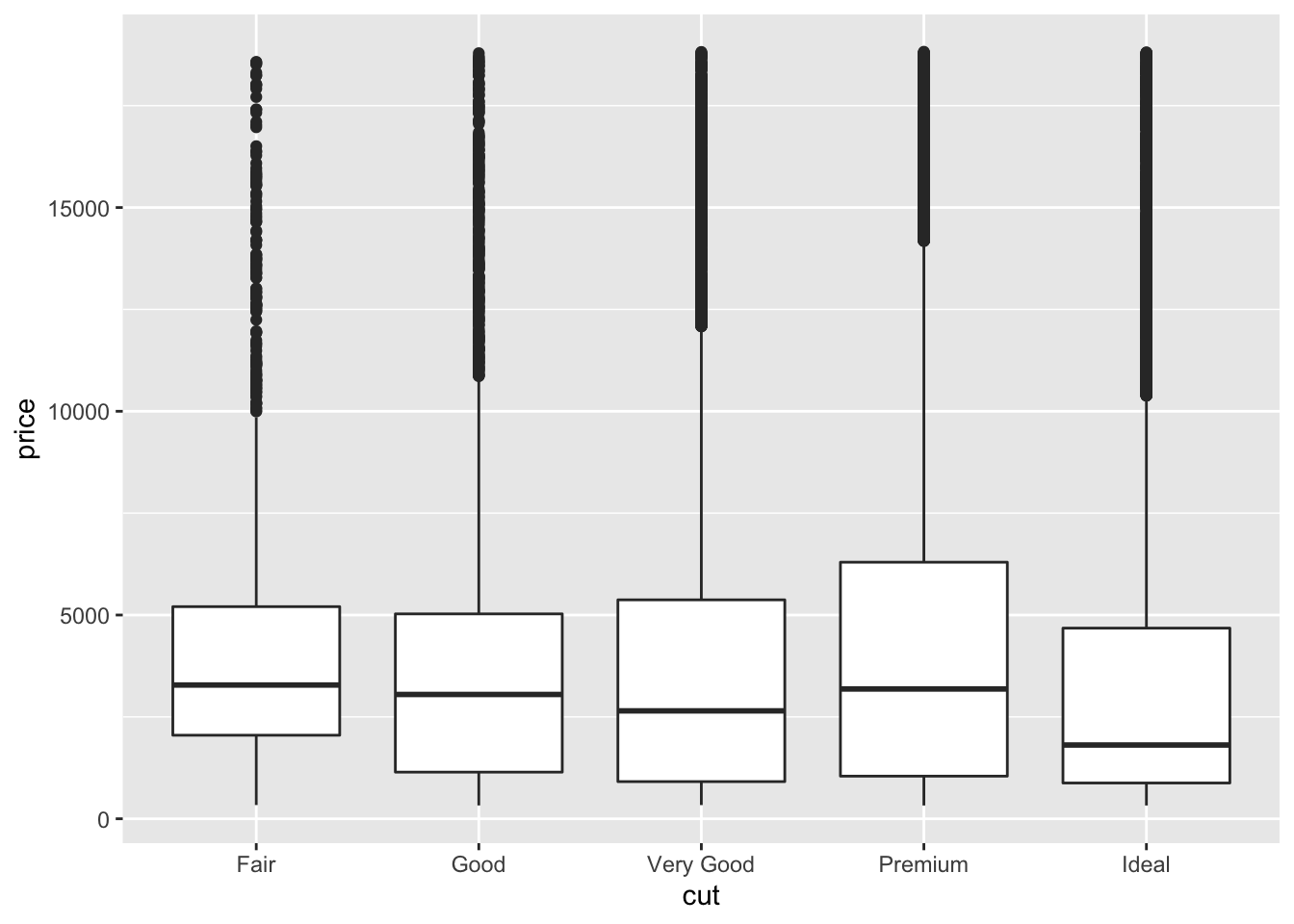 Please note: cut here is an ordered factor (whereby the plot automatically orders from the lowest quality = fair, to the highest = ideal). This is not always the case for categorical variables (or factors). For example:
ggplot(data = mpg, mapping = aes(x = class, y = hwy)) +
  geom_boxplot()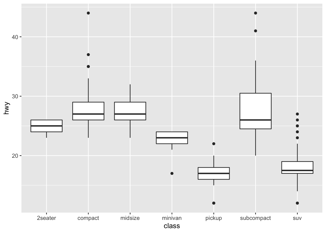
We can reorder them easily, for example by the median:
ggplot(data = mpg) +
geom_boxplot(mapping = aes(x = reorder(class, hwy, FUN = median), y = hwy)) #here we could order then on other things like the mean, too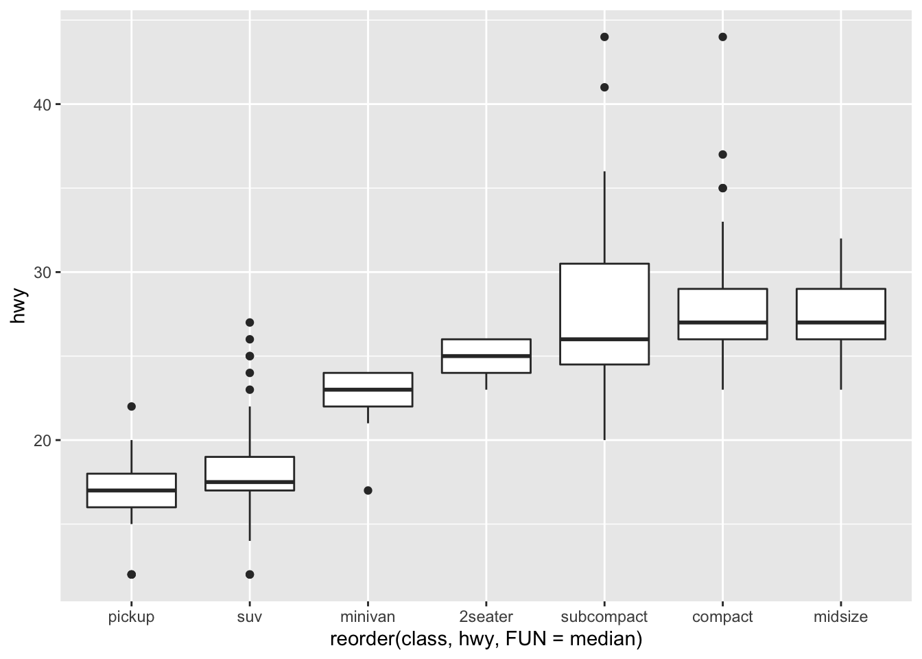 Hence, you can start to see patterns and relationships between the categorical variables with continuous ones.
4.2.6.2 Two Categorial Variables
You can look at the covariance between categorical variables by counting them, as we have done earlier using the dplyr package:
diamonds %>%
  dplyr::count(color, cut)
## # A tibble: 35 × 3
## color cut n
## <ord> <ord> <int>
## 1 D Fair 163
## 2 D Good 662
## 3 D Very Good 1513
## 4 D Premium 1603
## 5 D Ideal 2834
## 6 E Fair 224
## 7 E Good 933
## 8 E Very Good 2400
## 9 E Premium 2337
## 10 E Ideal 3903
## # … with 25 more rowsWe could also visualize this using a heatmap (known as geom_tile), which is a really nice way to visualize this:
diamonds %>%
  dplyr::count(color, cut) %>%
  ggplot(mapping = aes(x = color, y = cut)) +
    geom_tile(mapping = aes(fill = n))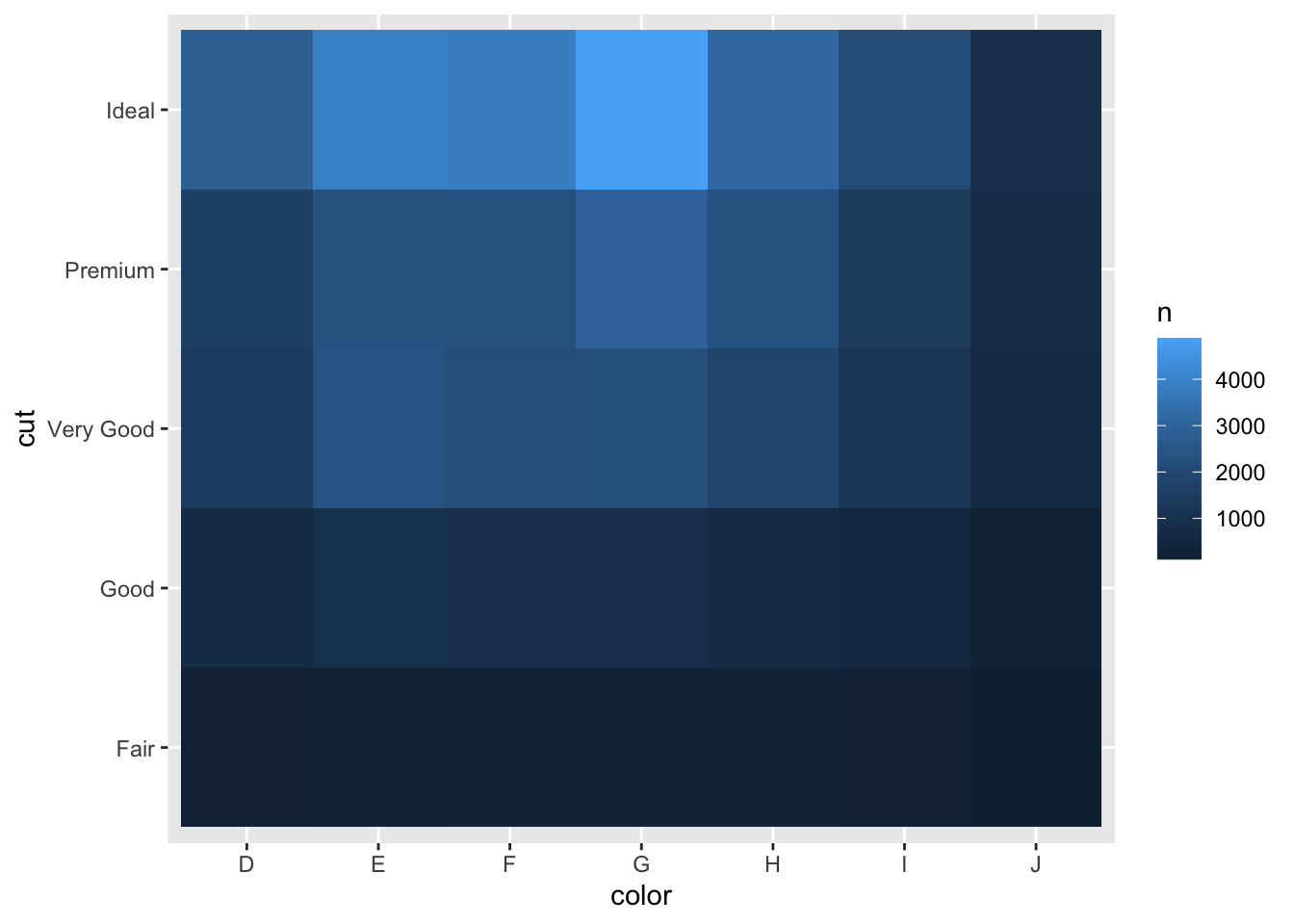
4.2.6.3 Two Continuous Variables
The classic way to look at continuous variables is to use a scatter plot, which will also give you an idea as to the correlations in the dataset, too. For example, there is an exponential relationship in the diamonds dataset when looking at carat size and price:
ggplot(data = diamonds) +
geom_point(mapping = aes(x = carat, y = price))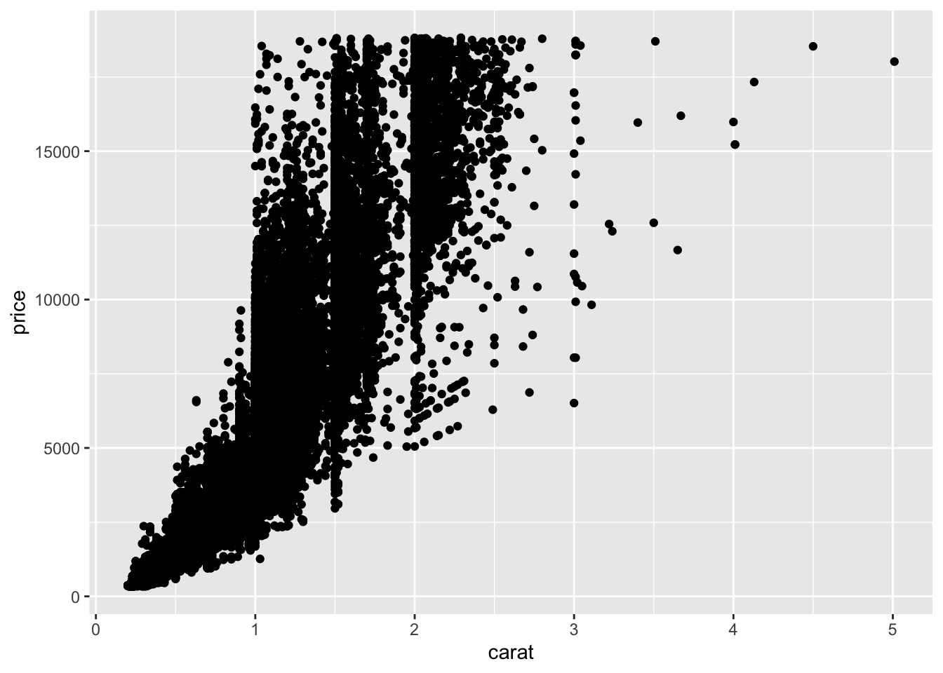 Similarly, there is not always an obvious relationship, where the correlation/relationship between Sepal Length and Width is less clear.
ggplot(iris, aes(Sepal.Width, Sepal.Length)) +
  geom_point()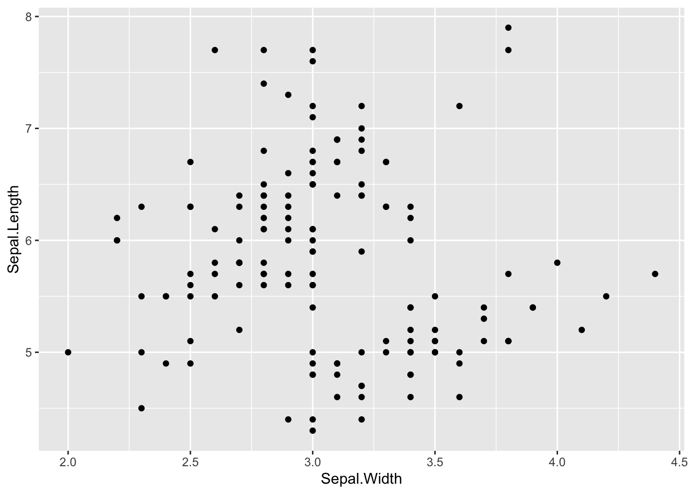
4.3 Missing Data
Sometimes when you collect data or are analyzing secondary data, there are missing values. This can appear as NULL or NA, and sometimes in other ways, it is good to check for these straight away. Missing values are considered to be the first obstacle in (predictive) modeling. Hence, it’s important to consider the variety of methods to handle them. Please note, some of the methods here jump to rather advanced statistics, while I do not go into the numbers beyond conceptually, please be aware of this before you start employing these methods. It is important to know why you’re doing this first and checking whether these methods are appropriate. These sections will be expanded more with time.
4.3.1 NA v NULL in R
Focusing on R… there are two similar but different types of missing value, NA and NULL – what is the difference? Well, the documentation for R states:
NULL represents the null object in R: it is a reserved word. NULL is often returned by expressions and functions whose values are undefined.
NA is a logical constant of length 1 which contains a missing value indicator. NA can be freely coerced to any other vector type except raw. There are also constants NA_integer_, NA_real_, NA_complex_ and NA_character_ of the other atomic vector types which support missing values: all of these are reserved words in the R language.
While there are subtle differences, R is not always consistent with how it works. Please be careful. (To be expanded…)
4.3.2 So, what do we do?
Well, thankfully there are a large choice of methods to impute missing values, largely influences the model’s predictive ability. In most statistical analysis methods, ‘listwise deletion’ is the default method used to impute missing values. By this, I mean we delete the entire record/row/observation from the dataset of any of the columns/variables are incomplete. But, it not as good since it leads to information loss… however, there are other ways we can handle missing values.
There are a couple of very simple ways you can quickly handle this without imputation:
- Remove any missing data observations (listwise deletion) – most common method (not necessarily the most sensible, either…):
 #Let's look at the iris dataset and randomly add in some missing values to demonstrate (as the original dataset does not have any missing values)
library('mice') #package for imputations
library('missForest') #another package for imputations and has a command to induce missing values
iris_missing <- prodNA(iris, noNA = 0.1) #creating 10% missing values
head(iris_missing)
## Sepal.Length Sepal.Width Petal.Length Petal.Width Species
## 1 5.1 3.5 1.4 0.2 setosa
## 2 4.9 3.0 1.4 0.2 setosa
## 3 4.7 NA 1.3 0.2 setosa
## 4 4.6 3.1 1.5 0.2 setosa
## 5 NA 3.6 NA 0.2 setosa
## 6 5.4 3.9 1.7 0.4 setosa#hopefully when you use the head() function you will see some of the missing values, if not call the dataset and check they are thereSo we have induced NA values into the iris dataset, let’s just remove them (there are many ways to do this, this is just one)
iris_remove_missing <- na.omit(iris_missing)

dim(iris_remove_missing) #get the dimnensions of the new dataframe
## [1] 85 5So, you should see here that there are far fewer rows of data, as we removed a number of them to remove NA values. This is a valid method for handling missing values, but this does mean we might have far less data left over. Similarly, the issue here is that we might find that we are removing important participants, so this might be an extreme option. Think critically about whether this is the right decision for your data and research questions.
- Leave them in:
This is an important other option, where you leave the data alone and continue with missing values. If you do this, be careful with how various commands handle missing values… for example, ggplot2 does not know where to plot missing values, so ggplot2 doesn’t include them in the plot, but it does warn that they’ve been removed:
ggplot(iris_missing, aes(Sepal.Length, Sepal.Width)) +
  geom_point()
## Warning: Removed 29 rows containing missing values (geom_point).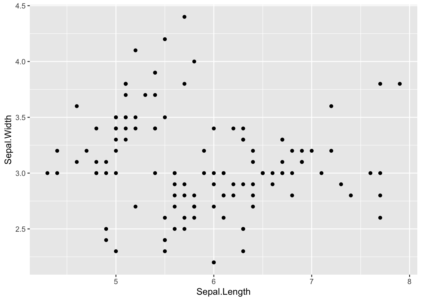
# where the warning states: Removed 30 rows containing missing values (geom_point).
#please note this might be a different number to you because we RANDOMLY added in NA values, so do not worry!
There are times where you will want to keep in missing data, for example, in the flights dataset, a missing value in departure time (dep_time) indicates a flight was cancelled. Therefore, be careful for whenever you decide to remove or leave in missing data!
library('nycflights13')

flights %>%
  mutate(
    cancelled = is.na(dep_time),
    sched_hour = sched_dep_time %/% 100,
    sched_min = sched_dep_time %% 100,
    sched_dep_time = sched_hour + sched_min / 60
  ) %>%
  ggplot(mapping = aes(sched_dep_time)) +
    geom_freqpoly(mapping = aes(colour = cancelled), binwidth = 1/4)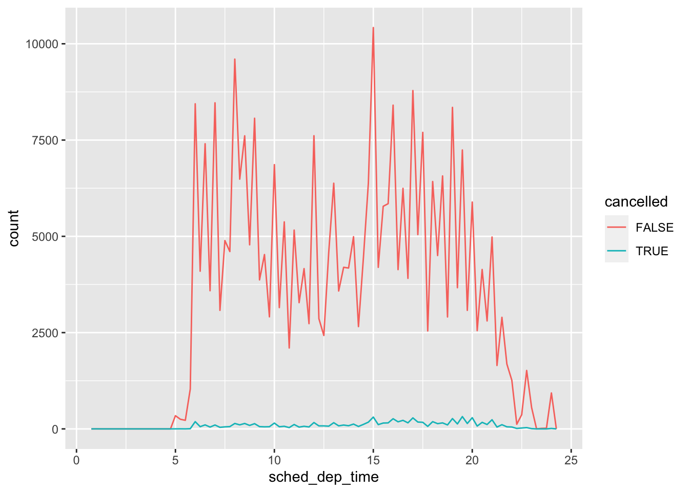
4.4 Imputations
We are luck that in R there are a number of packages build to handle imputations. For example: 1. Mice
Amelia
missForest
This is not an exhaustive list! There are more! We will look at a couple of these as an example to see how we can impute missing values. There are a number of considerations when doing this, rather than employing a ‘listwise deletion’. For example, are the missing values random? This is an extremely important question as this inherently means we would handle the imputations differently…and sometimes this is hard to know.
4.4.1 Definitions
Let’s dsicuss the different types of missing data briefly. Definitions are taken from ]this paper] (https://www.tandfonline.com/doi/pdf/10.1080/08839514.2019.1637138?casa_token=HlDOGucxnF4AAAAA:kMM2t7SeZ4fRedtfAsyXw0BuJB3pxzLEdE5wrrc_L1cusq75SuAtvBySQiiSDzjdgvWNn1LfLwQ):
Missing Completely at Random (MCAR): MCAR is the highest level of randomness and it implies that the pattern of missing value is totally random and does not depend on any variable which may or may not be included in the analysis. Thus, if missingness does not depend on any information in the dataset then it means that data is missing completely at random. The assumption of MCAR isthat probability of the missingness depends neither on the observed values in any variable of the dataset nor on unobserved part of dataset.
Missing at Random (MAR): In this case, probability of missing data is dependent on observed information in the dataset. It means that probability of missingness depends on observed information but does not depend on the unobserved part. Missing value of any of the variable in the dataset depends on observed values of other variables in the dataset because some correlation exists between attribute containing missing value and other attributes in the dataset. The pattern of missing data may be traceable from the observed values in the dataset.
Missing Not at Random (MNAR): In this case, missingness is dependent on unobserved data rather than observed data. Missingness depends on missing data or item itself because of response variable is too sensitive to answer. When data are MNAR, the probability of missing data is related to the value of the missing data itself. The pattern of missing data is not random and is non predictable from observed values of the other variables in the dataset.
4.4.2 Imputation Examples
4.4.2.1 [Mice package] (https://cran.r-project.org/web/packages/mice/mice.pdf)
MICE (Multivariate Imputation via Chained Equations) assumes that the missing data are Missing at Random (MAR), which means that the probability that a value is missing depends only on observed value and can be predicted using them. It imputes data on a variable by variable basis by specifying an imputation model per variable.
By default, linear regression is used to predict continuous missing values. Logistic regression is used for categorical missing values. Once this cycle is complete, multiple data sets are generated. These data sets differ only in imputed missing values. Generally, it’s considered to be a good practice to build models on these data sets separately and combining their results.
Precisely, the methods used by this package are:
PMM (Predictive Mean Matching) – For numeric variables
logreg(Logistic Regression) – For Binary Variables( with 2 levels)
polyreg(Bayesian polytomous regression) – For Factor Variables (>= 2 levels)
Proportional odds model (ordered, >= 2 levels)
We will use the missing iris data we creative above (iris_missing). First, for the sake of simplicity, we will remove the Species variable (categorial):
iris_missing <- subset(iris_missing,
                       select = -c(Species))

summary(iris_missing)
## Sepal.Length Sepal.Width Petal.Length Petal.Width
## Min. :4.300 Min. :2.200 Min. :1.000 Min. :0.100
## 1st Qu.:5.100 1st Qu.:2.800 1st Qu.:1.600 1st Qu.:0.300
## Median :5.800 Median :3.000 Median :4.500 Median :1.300
## Mean :5.865 Mean :3.077 Mean :3.893 Mean :1.233
## 3rd Qu.:6.400 3rd Qu.:3.400 3rd Qu.:5.200 3rd Qu.:1.800
## Max. :7.900 Max. :4.400 Max. :6.900 Max. :2.500
## NA's :14 NA's :15 NA's :17 NA's :13We installed and loaded Mice above, so we do not need to do that again. We will first use the command md.pattern(), which returns a table of the missing values in each dataset.
md.pattern(iris_missing, plot = FALSE)## Petal.Width Sepal.Length Sepal.Width Petal.Length
## 94 1 1 1 1 0
## 14 1 1 1 0 1
## 15 1 1 0 1 1
## 12 1 0 1 1 1
## 2 1 0 1 0 2
## 12 0 1 1 1 1
## 1 0 1 1 0 2
## 13 14 15 17 59[Insert Week2_Fig1 here as a static image] Referring to the static figure as the numbers will change each time the code is run… Let’s read it together.
Take the first row, reading from left to right: there are 104 observations with no missing values. Take the second row, there are 12 observations with missing values in Petal.Length. Take the third row, there are 9 missing values with Sepal.Length, and so on.
Take the above code and try running this with ‘plot = TRUE’ and see how the output changes.
Let impute the values. Here are the parameters used in this example:
m– Refers to 5 imputed data setsmaxit– Refers to number of iterations taken to impute missing valuesmethod– Refers to method used in imputation, where we used predictive mean matching.
imputed_Data <- mice(iris_missing, m=5, maxit = 50, method = 'pmm', seed = 500)

summary(imputed_Data)
We can look and check our newly imputed data (note there are 5 columns as it created 5 new datasets:
imputed_Data$imp$Sepal.Length## 1 2 3 4 5
## 5 5.4 5.4 5.8 4.7 5.2
## 7 5.0 4.7 4.8 4.6 5.0
## 10 5.0 5.1 4.8 4.6 4.6
## 25 5.5 5.5 5.7 5.2 4.9
## 42 4.8 5.0 4.3 4.3 4.9
## 64 6.1 6.4 6.8 6.1 6.8
## 68 6.4 5.8 5.8 6.0 5.8
## 96 5.4 5.8 6.6 6.6 6.0
## 99 5.0 5.4 5.0 5.0 5.0
## 109 6.9 6.8 7.0 6.7 6.5
## 111 6.3 6.7 6.3 6.9 7.0
## 124 6.0 6.2 6.0 5.8 5.6
## 142 6.0 6.3 5.8 6.4 6.0
## 150 6.3 6.7 6.7 6.3 6.9Let’s take the 3rd dataset and use this…
completeData <- complete(imputed_Data, 3) #3 signifies the 3rd dataset

head(completeData) #preview of the new complete dataset, where there will be no more missing values
## Sepal.Length Sepal.Width Petal.Length Petal.Width
## 1 5.1 3.5 1.4 0.2
## 2 4.9 3.0 1.4 0.2
## 3 4.7 3.2 1.3 0.2
## 4 4.6 3.1 1.5 0.2
## 5 5.8 3.6 1.6 0.2
## 6 5.4 3.9 1.7 0.44.4.2.2 [Amelia Package] (https://cran.r-project.org/web/packages/Amelia/Amelia.pdf)
This package also performs multiple imputation (generate imputed datasets) to deal with missing values. Multiple imputation helps to reduce bias and increase efficiency. It is enabled with the bootstrap based EMB algorithm, which makes it faster and robust to impute many variables including cross sectional, time series data etc. Also, it is enabled with parallel imputation feature using multicore CPUs.
This package also assumes:
All variables in a data set have Multivariate Normal Distribution (MVN). It uses means and covariances to summarize data. So please please check your data for skews/normality before you use this!
Missing data is random in nature (Missing at Random)
What’s the difference between Ameila with Mice?
Mice imputes data on variable by variable basis whereas MVN (Amelia) uses a joint modeling approach based on multivariate normal distribution.
Mice is capable of handling different types of variables whereas the variables in MVN (Ameila) need to be normally distributed or transformed to approximate normality.
Mice can manage imputation of variables defined on a subset of data whereas MVN (Amelia) cannot.
Let’s have a go (and create a new iris missing dataset that keeps the categorical species variable)
library('Amelia')

iris_missing2 <- prodNA(iris, noNA = 0.15) #taking iris dataset and adding in 15% missing values
head(iris_missing2)
## Sepal.Length Sepal.Width Petal.Length Petal.Width Species
## 1 NA 3.5 1.4 0.2 <NA>
## 2 4.9 3.0 1.4 0.2 setosa
## 3 4.7 3.2 1.3 0.2 setosa
## 4 NA 3.1 1.5 0.2 setosa
## 5 5.0 NA NA 0.2 setosa
## 6 5.4 3.9 1.7 0.4 setosaWhen using Ameila, we need to specify some arguments. First: idvars = keep all ID variables and others that we do not want to impute, and second: noms = we want to keep all nominal/categorical variables.
amelia_fit <- amelia(iris_missing2, m=5, parallel = 'multicore', noms = 'Species')## -- Imputation 1 --
##
## 1 2 3 4 5 6 7 8 9
##
## -- Imputation 2 --
##
## 1 2 3 4 5 6 7 8
##
## -- Imputation 3 --
##
## 1 2 3 4 5 6 7 8
##
## -- Imputation 4 --
##
## 1 2 3 4 5 6 7 8 9
##
## -- Imputation 5 --
##
## 1 2 3 4 5 6 7Lets look at the imputed datasets
amelia_fit$imputations[[1]]
amelia_fit$imputations[[2]]
amelia_fit$imputations[[3]]
amelia_fit$imputations[[4]]
amelia_fit$imputations[[5]]
Here we can see each of the newdaatframes, and we can use the $ to look at specific variables too.You can write these to .csv files by using: write.amelia(amelia_fit, file.stem = “imputed_data_set”) for example.
4.4.2.3 [missForest] (https://cran.r-project.org/web/packages/missForest/missForest.pdf)
missForest is an implementation of random forest algorithm, which you will learn more about in the Machine Learning Unit if you’ve not taken it already. Broadly, this will be a non parametric imputation method applicable to various variable types. To recap, non-parametric method does not make explicit assumptions about data distributions (e.g., if you data are skewed or non-normal, that is OK). Instead, it tries to estimate f such that it can be as close to the data points without seeming impractical. Essentially, missForest builds a random forest model for each variable to then use the model to predict missing values in the variable with the help of observed values.
Let’s have a go! (we have installed and loaded missForest already, if you haven’t load it!)
#we will use the missing data we used in the Amelia example (iris_missing2)

#lets impute missing values, using all parameters
iris_imputed <- missForest(iris_missing2)
## missForest iteration 1 in progress...done!
## missForest iteration 2 in progress...done!
## missForest iteration 3 in progress...done!
## missForest iteration 4 in progress...done!Lets check the imputed values…
#check imputed values
iris_imputed$ximp
Lets look at the prediction error. This gives you two values: the NRMSE and the PFC. The NRMSE is the normalized mean squared error. It is used to represent error derived from imputing continuous values. The PFC (proportion of falsely classified) is used to represent error derived from imputing categorical values.
iris_imputed$OOBerror## NRMSE PFC
## 0.14489524 0.02307692Finally, we can compare the actual data accuracy (using original iris dataset)
iris_error <- mixError(iris_imputed$ximp, iris_missing2, iris)

iris_error
## NRMSE PFC
## 0.1399269 0.1000000#output (remember this will change each time you run it, for the sake of explaining the output I've commented it!)
#NRMSE PFC
#0.15547993 0.04761905 Noting data and outcomes will change as we are randomly inducing missing values, in this example, the NRMSE is 0.156 and the PFC is 0.048. This suggests that categorical variables are imputed with 4.8% error and continuous variables are imputed with 15.6% error.
4.5 Basic Statistics in R
This will recap the main ways to do descriptive statistics in R. This is not a chapter in how to do statistics, as this has already been covered in earlier modules. However, if you’d like a deep dive into statistics, I’d recommend: https://www.coursera.org/instructor/~20199472.
With a lot of things you can do in the R programming language, there are a number of ways to do the same thing. Hence, here, we will look at a number of different coding styles, too, drawing on the ‘tidy’ way, among base R across a number of packages.
For this, we will use the iris dataset. PLEASE BE CAREFUL OF WHICH PACKAGE YOU ARE CALLING DUE TO COMMANDS WITH THE SAME NAME. This is a common issue that will break your code. For example, if you want to use describe() – do you want the psych package or Hmisc? Ensure you know your packages and how they overlap in command names and also whether one package masks another (e.g., sometimes the order of package loading is important…)
4.5.1 Descriptive Statistics
One of the simplest ways to capture descriptives from a dataframe uses the summary() function in base R. This provides: mean, median, 25th and 75th quartiles, min, and max values:
#loading typical packages just in case you've not already
library('dplyr')
library('magrittr')
library('ggplot2')
library('tidyverse')

head(iris) #ensure you've loaded packages and iris is accessible
## Sepal.Length Sepal.Width Petal.Length Petal.Width Species
## 1 5.1 3.5 1.4 0.2 setosa
## 2 4.9 3.0 1.4 0.2 setosa
## 3 4.7 3.2 1.3 0.2 setosa
## 4 4.6 3.1 1.5 0.2 setosa
## 5 5.0 3.6 1.4 0.2 setosa
## 6 5.4 3.9 1.7 0.4 setosa#lets get the means for variables in iris
# we will exclude missing values
base::summary(iris)## Sepal.Length Sepal.Width Petal.Length Petal.Width Species
## Min. :4.300 Min. :2.000 Min. :1.000 Min. :0.100 setosa :50
## 1st Qu.:5.100 1st Qu.:2.800 1st Qu.:1.600 1st Qu.:0.300 versicolor:50
## Median :5.800 Median :3.000 Median :4.350 Median :1.300 virginica :50
## Mean :5.843 Mean :3.057 Mean :3.758 Mean :1.199
## 3rd Qu.:6.400 3rd Qu.:3.300 3rd Qu.:5.100 3rd Qu.:1.800
## Max. :7.900 Max. :4.400 Max. :6.900 Max. :2.500This of course provides a variety of statistics that may be of use. Similarly, the Hmisc package provides some useful and more detailed statistics that includes: n, number of missing values, number of unique values (disctinct), mean, 5, 10, 25, 50, 75, 90, 95th percentiles, 5 lowest and 5 highest scores:
library('Hmisc')

Hmisc::describe(iris) #make sure this command is coming from the Hmisc package
## iris
##
## 5 Variables 150 Observations
## -------------------------------------------------------------------------------------------------------------------------------------------------
## Sepal.Length
## n missing distinct Info Mean Gmd .05 .10 .25 .50 .75 .90 .95
## 150 0 35 0.998 5.843 0.9462 4.600 4.800 5.100 5.800 6.400 6.900 7.255
##
## lowest : 4.3 4.4 4.5 4.6 4.7, highest: 7.3 7.4 7.6 7.7 7.9
## -------------------------------------------------------------------------------------------------------------------------------------------------
## Sepal.Width
## n missing distinct Info Mean Gmd .05 .10 .25 .50 .75 .90 .95
## 150 0 23 0.992 3.057 0.4872 2.345 2.500 2.800 3.000 3.300 3.610 3.800
##
## lowest : 2.0 2.2 2.3 2.4 2.5, highest: 3.9 4.0 4.1 4.2 4.4
## -------------------------------------------------------------------------------------------------------------------------------------------------
## Petal.Length
## n missing distinct Info Mean Gmd .05 .10 .25 .50 .75 .90 .95
## 150 0 43 0.998 3.758 1.979 1.30 1.40 1.60 4.35 5.10 5.80 6.10
##
## lowest : 1.0 1.1 1.2 1.3 1.4, highest: 6.3 6.4 6.6 6.7 6.9
## -------------------------------------------------------------------------------------------------------------------------------------------------
## Petal.Width
## n missing distinct Info Mean Gmd .05 .10 .25 .50 .75 .90 .95
## 150 0 22 0.99 1.199 0.8676 0.2 0.2 0.3 1.3 1.8 2.2 2.3
##
## lowest : 0.1 0.2 0.3 0.4 0.5, highest: 2.1 2.2 2.3 2.4 2.5
## -------------------------------------------------------------------------------------------------------------------------------------------------
## Species
## n missing distinct
## 150 0 3
##
## Value setosa versicolor virginica
## Frequency 50 50 50
## Proportion 0.333 0.333 0.333
## -------------------------------------------------------------------------------------------------------------------------------------------------Similarly, we’ll look at the pastecs package, which gives you nbr.val, nbr.null, nbr.na, min max, range, sum, median, mean, SE.mean, CI.mean, var, std.dev, and coef.var as a series of more advanced statistics.
library('pastecs')

stat.desc(iris)
## Sepal.Length Sepal.Width Petal.Length Petal.Width Species
## nbr.val 150.00000000 150.00000000 150.0000000 150.00000000 NA
## nbr.null 0.00000000 0.00000000 0.0000000 0.00000000 NA
## nbr.na 0.00000000 0.00000000 0.0000000 0.00000000 NA
## min 4.30000000 2.00000000 1.0000000 0.10000000 NA
## max 7.90000000 4.40000000 6.9000000 2.50000000 NA
## range 3.60000000 2.40000000 5.9000000 2.40000000 NA
## sum 876.50000000 458.60000000 563.7000000 179.90000000 NA
## median 5.80000000 3.00000000 4.3500000 1.30000000 NA
## mean 5.84333333 3.05733333 3.7580000 1.19933333 NA
## SE.mean 0.06761132 0.03558833 0.1441360 0.06223645 NA
## CI.mean.0.95 0.13360085 0.07032302 0.2848146 0.12298004 NA
## var 0.68569351 0.18997942 3.1162779 0.58100626 NA
## std.dev 0.82806613 0.43586628 1.7652982 0.76223767 NA
## coef.var 0.14171126 0.14256420 0.4697441 0.63555114 NAFinally, the psych package is very common for social science scholars, which provides another series of descriptive outputs that include: item name, item number, nvalid, mean, sd, median, mad, min, max, skew, kurtosis, and se:
library(psych)

psych::describe(iris) #calling psych:: to ensure we are using the correct package
## vars n mean sd median trimmed mad min max range skew kurtosis se
## Sepal.Length 1 150 5.84 0.83 5.80 5.81 1.04 4.3 7.9 3.6 0.31 -0.61 0.07
## Sepal.Width 2 150 3.06 0.44 3.00 3.04 0.44 2.0 4.4 2.4 0.31 0.14 0.04
## Petal.Length 3 150 3.76 1.77 4.35 3.76 1.85 1.0 6.9 5.9 -0.27 -1.42 0.14
## Petal.Width 4 150 1.20 0.76 1.30 1.18 1.04 0.1 2.5 2.4 -0.10 -1.36 0.06
## Species* 5 150 2.00 0.82 2.00 2.00 1.48 1.0 3.0 2.0 0.00 -1.52 0.07Another useful element of the psych package is that you can describe by group, whereby we can get the same descriptive statistics as above, but specifically for each species:
describeBy(iris, group = 'Species')##
## Descriptive statistics by group
## Species: setosa
## vars n mean sd median trimmed mad min max range skew kurtosis se
## Sepal.Length 1 50 5.01 0.35 5.0 5.00 0.30 4.3 5.8 1.5 0.11 -0.45 0.05
## Sepal.Width 2 50 3.43 0.38 3.4 3.42 0.37 2.3 4.4 2.1 0.04 0.60 0.05
## Petal.Length 3 50 1.46 0.17 1.5 1.46 0.15 1.0 1.9 0.9 0.10 0.65 0.02
## Petal.Width 4 50 0.25 0.11 0.2 0.24 0.00 0.1 0.6 0.5 1.18 1.26 0.01
## Species* 5 50 1.00 0.00 1.0 1.00 0.00 1.0 1.0 0.0 NaN NaN 0.00
## ------------------------------------------------------------------------------------------------------------
## Species: versicolor
## vars n mean sd median trimmed mad min max range skew kurtosis se
## Sepal.Length 1 50 5.94 0.52 5.90 5.94 0.52 4.9 7.0 2.1 0.10 -0.69 0.07
## Sepal.Width 2 50 2.77 0.31 2.80 2.78 0.30 2.0 3.4 1.4 -0.34 -0.55 0.04
## Petal.Length 3 50 4.26 0.47 4.35 4.29 0.52 3.0 5.1 2.1 -0.57 -0.19 0.07
## Petal.Width 4 50 1.33 0.20 1.30 1.32 0.22 1.0 1.8 0.8 -0.03 -0.59 0.03
## Species* 5 50 2.00 0.00 2.00 2.00 0.00 2.0 2.0 0.0 NaN NaN 0.00
## ------------------------------------------------------------------------------------------------------------
## Species: virginica
## vars n mean sd median trimmed mad min max range skew kurtosis se
## Sepal.Length 1 50 6.59 0.64 6.50 6.57 0.59 4.9 7.9 3.0 0.11 -0.20 0.09
## Sepal.Width 2 50 2.97 0.32 3.00 2.96 0.30 2.2 3.8 1.6 0.34 0.38 0.05
## Petal.Length 3 50 5.55 0.55 5.55 5.51 0.67 4.5 6.9 2.4 0.52 -0.37 0.08
## Petal.Width 4 50 2.03 0.27 2.00 2.03 0.30 1.4 2.5 1.1 -0.12 -0.75 0.04
## Species* 5 50 3.00 0.00 3.00 3.00 0.00 3.0 3.0 0.0 NaN NaN 0.004.5.2 Correlations
Correlation or dependence is any statistical relationship, whether causal or not (this is important!), between two random variables or bivariate data. In the broadest sense, a correlation is any statistical association between two variables, though it commonly refers to the degree to which a pair of variables are linearly related.
Thre are a number of ways we can capture a correlation both numerically or visually. For instance, in base R we can use cor() to get the correlation. You can define the method: perason, spearman, or kendall. However, if you’d like to see the p-value, you’d need to use the cor.test() function to get the correlation coefficient. Similarly, using the Hmisc package, the rcorr() command produces correlations, covariances, and significance levels for pearson and spearman correlations. Lets have a look:
cor(mtcars, use = "everything", method ="pearson")## mpg cyl disp hp drat wt qsec vs am gear carb
## mpg 1.0000000 -0.8521620 -0.8475514 -0.7761684 0.68117191 -0.8676594 0.41868403 0.6640389 0.59983243 0.4802848 -0.55092507
## cyl -0.8521620 1.0000000 0.9020329 0.8324475 -0.69993811 0.7824958 -0.59124207 -0.8108118 -0.52260705 -0.4926866 0.52698829
## disp -0.8475514 0.9020329 1.0000000 0.7909486 -0.71021393 0.8879799 -0.43369788 -0.7104159 -0.59122704 -0.5555692 0.39497686
## hp -0.7761684 0.8324475 0.7909486 1.0000000 -0.44875912 0.6587479 -0.70822339 -0.7230967 -0.24320426 -0.1257043 0.74981247
## drat 0.6811719 -0.6999381 -0.7102139 -0.4487591 1.00000000 -0.7124406 0.09120476 0.4402785 0.71271113 0.6996101 -0.09078980
## wt -0.8676594 0.7824958 0.8879799 0.6587479 -0.71244065 1.0000000 -0.17471588 -0.5549157 -0.69249526 -0.5832870 0.42760594
## qsec 0.4186840 -0.5912421 -0.4336979 -0.7082234 0.09120476 -0.1747159 1.00000000 0.7445354 -0.22986086 -0.2126822 -0.65624923
## vs 0.6640389 -0.8108118 -0.7104159 -0.7230967 0.44027846 -0.5549157 0.74453544 1.0000000 0.16834512 0.2060233 -0.56960714
## am 0.5998324 -0.5226070 -0.5912270 -0.2432043 0.71271113 -0.6924953 -0.22986086 0.1683451 1.00000000 0.7940588 0.05753435
## gear 0.4802848 -0.4926866 -0.5555692 -0.1257043 0.69961013 -0.5832870 -0.21268223 0.2060233 0.79405876 1.0000000 0.27407284
## carb -0.5509251 0.5269883 0.3949769 0.7498125 -0.09078980 0.4276059 -0.65624923 -0.5696071 0.05753435 0.2740728 1.00000000#please note: under use, this allows you to specify how to use missing data, where all.obs = assumes no missing data
#and if there is missing data this will error; complete.obs will perform listwise deletion, etc.
#As above, if we wanted to see the correlation coefficients, using cor.test() is one way to do this.
#this provides correlation statistics for a SINGLE COEFFICIENT (see below)
cor.test(mtcars$mpg, mtcars$cyl)##
## Pearson's product-moment correlation
##
## data: mtcars$mpg and mtcars$cyl
## t = -8.9197, df = 30, p-value = 6.113e-10
## alternative hypothesis: true correlation is not equal to 0
## 95 percent confidence interval:
## -0.9257694 -0.7163171
## sample estimates:
## cor
## -0.852162#using Hmisc package
#note: input MUST be a matrix and pairwise deletion must have been useed
Hmisc::rcorr(as.matrix(mtcars))## mpg cyl disp hp drat wt qsec vs am gear carb
## mpg 1.00 -0.85 -0.85 -0.78 0.68 -0.87 0.42 0.66 0.60 0.48 -0.55
## cyl -0.85 1.00 0.90 0.83 -0.70 0.78 -0.59 -0.81 -0.52 -0.49 0.53
## disp -0.85 0.90 1.00 0.79 -0.71 0.89 -0.43 -0.71 -0.59 -0.56 0.39
## hp -0.78 0.83 0.79 1.00 -0.45 0.66 -0.71 -0.72 -0.24 -0.13 0.75
## drat 0.68 -0.70 -0.71 -0.45 1.00 -0.71 0.09 0.44 0.71 0.70 -0.09
## wt -0.87 0.78 0.89 0.66 -0.71 1.00 -0.17 -0.55 -0.69 -0.58 0.43
## qsec 0.42 -0.59 -0.43 -0.71 0.09 -0.17 1.00 0.74 -0.23 -0.21 -0.66
## vs 0.66 -0.81 -0.71 -0.72 0.44 -0.55 0.74 1.00 0.17 0.21 -0.57
## am 0.60 -0.52 -0.59 -0.24 0.71 -0.69 -0.23 0.17 1.00 0.79 0.06
## gear 0.48 -0.49 -0.56 -0.13 0.70 -0.58 -0.21 0.21 0.79 1.00 0.27
## carb -0.55 0.53 0.39 0.75 -0.09 0.43 -0.66 -0.57 0.06 0.27 1.00
##
## n= 32
##
##
## P
## mpg cyl disp hp drat wt qsec vs am gear carb
## mpg 0.0000 0.0000 0.0000 0.0000 0.0000 0.0171 0.0000 0.0003 0.0054 0.0011
## cyl 0.0000 0.0000 0.0000 0.0000 0.0000 0.0004 0.0000 0.0022 0.0042 0.0019
## disp 0.0000 0.0000 0.0000 0.0000 0.0000 0.0131 0.0000 0.0004 0.0010 0.0253
## hp 0.0000 0.0000 0.0000 0.0100 0.0000 0.0000 0.0000 0.1798 0.4930 0.0000
## drat 0.0000 0.0000 0.0000 0.0100 0.0000 0.6196 0.0117 0.0000 0.0000 0.6212
## wt 0.0000 0.0000 0.0000 0.0000 0.0000 0.3389 0.0010 0.0000 0.0005 0.0146
## qsec 0.0171 0.0004 0.0131 0.0000 0.6196 0.3389 0.0000 0.2057 0.2425 0.0000
## vs 0.0000 0.0000 0.0000 0.0000 0.0117 0.0010 0.0000 0.3570 0.2579 0.0007
## am 0.0003 0.0022 0.0004 0.1798 0.0000 0.0000 0.2057 0.3570 0.0000 0.7545
## gear 0.0054 0.0042 0.0010 0.4930 0.0000 0.0005 0.2425 0.2579 0.0000 0.1290
## carb 0.0011 0.0019 0.0253 0.0000 0.6212 0.0146 0.0000 0.0007 0.7545 0.12904.5.3 Visual Correlations using corrplot
mtcars_mat <- cor(mtcars) #need to have the correlations to plot

corrplot::corrplot(mtcars_mat, method = 'ellipse', type = 'upper')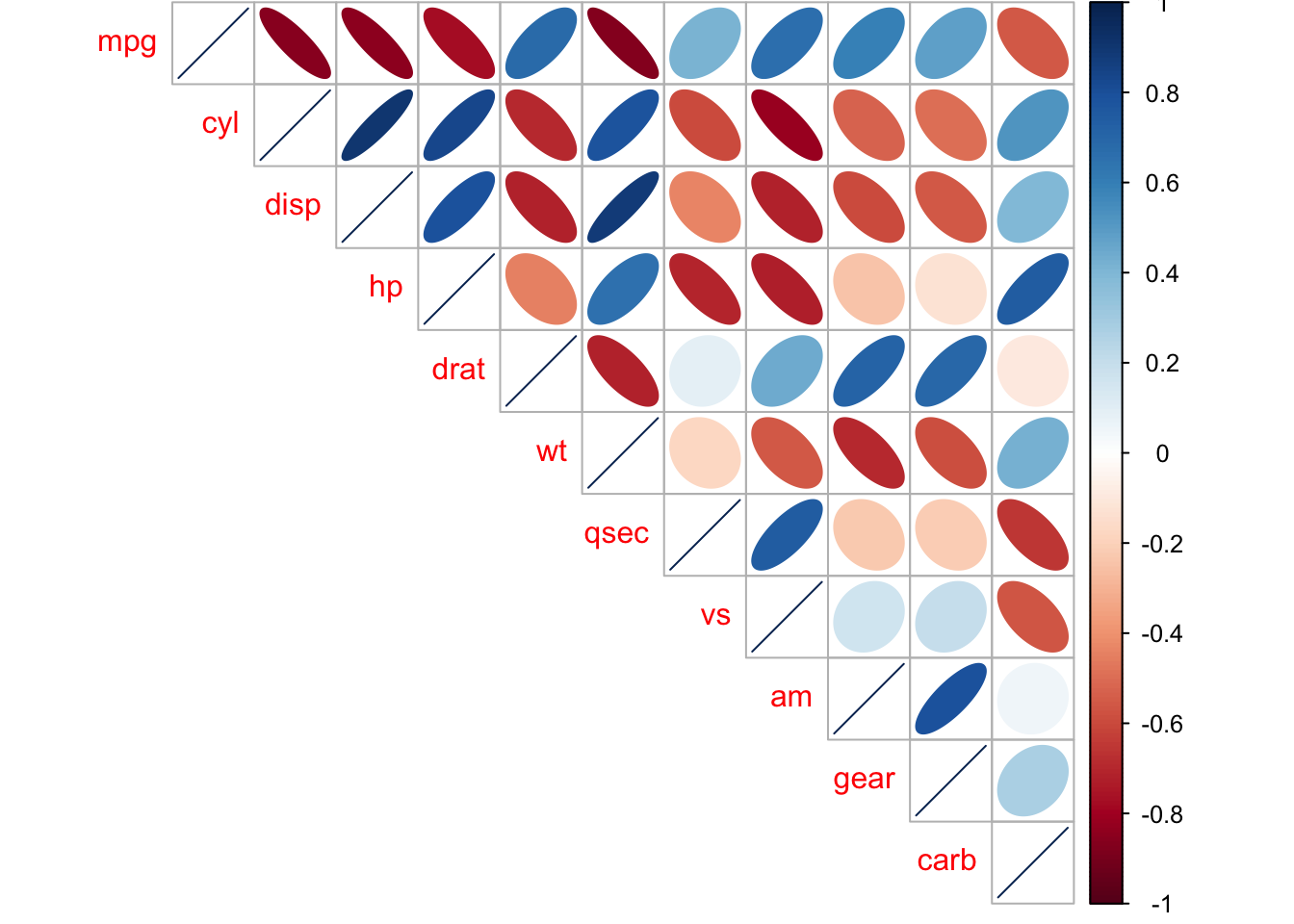
4.5.4 t-tests
t-tests compare two groups, for instance, control group and experimental groups. There are different types of t-tests, where the most common you’ll be looking at are independent t-tests or paired t-tests.
Briefly, an independent or unpaired t-test is when you’re comparing groups that are independent of one another, aka, each observation or participant was exposed to one of the groups only. For instance, in an exeriemtn you are only in the CONTROL or the EXPERIMENTAL condition.
In contrast, paired t-tests or repeated measures t-tests is where the participants are in BOTH groups, typically this is where participants are tested on one day and tested again at a later time. For example, you might be analyzing anxiety at the start of the week (Monday) versus the end of the week (Friday), so you ask participant to fill out the GAD7 on Monday and again on Friday and compare the difference.
4.5.4.1 Independent Samples t-test
Let’s create a dataset to use for an INDEPENDENT samples t-test:
# Data in two numeric vectors
women_weight <- c(38.9, 61.2, 73.3, 21.8, 63.4, 64.6, 48.4, 48.8, 48.5)
men_weight <- c(67.8, 60, 63.4, 76, 89.4, 73.3, 67.3, 61.3, 62.4)

# Create a data frame
my_data <- data.frame(
                group = rep(c("Woman", "Man"), each = 9),
                weight = c(women_weight,  men_weight)
                )

#check
print(my_data)
## group weight
## 1 Woman 38.9
## 2 Woman 61.2
## 3 Woman 73.3
## 4 Woman 21.8
## 5 Woman 63.4
## 6 Woman 64.6
## 7 Woman 48.4
## 8 Woman 48.8
## 9 Woman 48.5
## 10 Man 67.8
## 11 Man 60.0
## 12 Man 63.4
## 13 Man 76.0
## 14 Man 89.4
## 15 Man 73.3
## 16 Man 67.3
## 17 Man 61.3
## 18 Man 62.4It is always important to do some descriptive summary statistics across groups:
group_by(my_data, group) %>%
  dplyr::summarise(
    count = n(),
    mean = mean(weight, na.rm = TRUE),
    sd = sd(weight, na.rm = TRUE)
  )
## # A tibble: 2 × 4
## group count mean sd
## <chr> <int> <dbl> <dbl>
## 1 Man 9 69.0 9.38
## 2 Woman 9 52.1 15.6#or we can of course use describeBy
describeBy(my_data, group = 'group')##
## Descriptive statistics by group
## group: Man
## vars n mean sd median trimmed mad min max range skew kurtosis se
## group* 1 9 1.00 0.00 1.0 1.00 0.0 1 1.0 0.0 NaN NaN 0.00
## weight 2 9 68.99 9.38 67.3 68.99 8.9 60 89.4 29.4 0.98 -0.28 3.13
## ------------------------------------------------------------------------------------------------------------
## group: Woman
## vars n mean sd median trimmed mad min max range skew kurtosis se
## group* 1 9 1.0 0.0 1.0 1.0 0.00 1.0 1.0 0.0 NaN NaN 0.0
## weight 2 9 52.1 15.6 48.8 52.1 18.38 21.8 73.3 51.5 -0.49 -0.89 5.2As you will know, there are a number of assumptions that need to be checked before doing t-tests (or any linear tests, e.g., regression). For instance:
are your data normally distributed?
do the two sampls have the same variances? (e.g., looking for homogenetity, where we do not want significant differences between variances)
Let’s check those assumptions. We will use the Shapiro-Wilk normality test to test for normality in each group, where the null hypothesis is that the data are normally distributed and the alternative hypothesis is that the data are not normally distributed.
We’ll use the functions with() and shapiro.test() to compute Shapiro-Wilk test for each group of samples (without splitting data into two using subset() and then using the shapiro.test() function).
# Shapiro-Wilk normality test for Men's weights
with(my_data, shapiro.test(weight[group == "Man"]))
##
## Shapiro-Wilk normality test
##
## data: weight[group == "Man"]
## W = 0.86425, p-value = 0.1066# Shapiro-Wilk normality test for Women's weights
with(my_data, shapiro.test(weight[group == "Woman"]))##
## Shapiro-Wilk normality test
##
## data: weight[group == "Woman"]
## W = 0.94266, p-value = 0.6101Here we can see that both groups have a p-value that are greater than 0.05 whereby we interpret that the distributions are nor significantly different from a normal distribution. We can assume normality.
TO check for homogeneity in variances, we’ll use var.test(), which is an F-test:
res.ftest <- var.test(weight ~ group, data = my_data)
res.ftest
##
## F test to compare two variances
##
## data: weight by group
## F = 0.36134, num df = 8, denom df = 8, p-value = 0.1714
## alternative hypothesis: true ratio of variances is not equal to 1
## 95 percent confidence interval:
## 0.08150656 1.60191315
## sample estimates:
## ratio of variances
## 0.3613398Here, the p-value of F-test is p = 0.1713596. It is greater than the significance level alpha = 0.05, whereby here is no significant difference between the variances of the two sets of data. Therefore, we can use the classic t-test witch assume equality of the two variances.
Now, we can go ahead and do a t-test:
#there are multiple ways you can write this code

# Compute t-test method one:
res <- t.test(weight ~ group, data = my_data, var.equal = TRUE)
res
##
## Two Sample t-test
##
## data: weight by group
## t = 2.7842, df = 16, p-value = 0.01327
## alternative hypothesis: true difference in means is not equal to 0
## 95 percent confidence interval:
## 4.029759 29.748019
## sample estimates:
## mean in group Man mean in group Woman
## 68.98889 52.10000# Compute t-test method two
res <- t.test(women_weight, men_weight, var.equal = TRUE)
res##
## Two Sample t-test
##
## data: women_weight and men_weight
## t = -2.7842, df = 16, p-value = 0.01327
## alternative hypothesis: true difference in means is not equal to 0
## 95 percent confidence interval:
## -29.748019 -4.029759
## sample estimates:
## mean of x mean of y
## 52.10000 68.98889Briefly, the p-value of the test is 0.01327, which is less than the significance level alpha = 0.05. Hence, we can conclude that men’s average weight is significantly different from women’s average weight.
4.5.4.2 Paired Sample t-test
Here, we will look at the paired sample t-test. Lets create a dataset:
# Weight of the mice before treatment
before <-c(200.1, 190.9, 192.7, 213, 241.4, 196.9, 172.2, 185.5, 205.2, 193.7)
# Weight of the mice after treatment
after <-c(392.9, 393.2, 345.1, 393, 434, 427.9, 422, 383.9, 392.3, 352.2)
# Create a data frame
my_data_paired <- data.frame(
                group = rep(c("before", "after"), each = 10),
                weight = c(before,  after)
                )

print(my_data_paired)
## group weight
## 1 before 200.1
## 2 before 190.9
## 3 before 192.7
## 4 before 213.0
## 5 before 241.4
## 6 before 196.9
## 7 before 172.2
## 8 before 185.5
## 9 before 205.2
## 10 before 193.7
## 11 after 392.9
## 12 after 393.2
## 13 after 345.1
## 14 after 393.0
## 15 after 434.0
## 16 after 427.9
## 17 after 422.0
## 18 after 383.9
## 19 after 392.3
## 20 after 352.2group_by(my_data_paired, group) %>%
dplyr::summarise(
count = n(),
mean = mean(weight, na.rm = TRUE),
sd = sd(weight, na.rm = TRUE)
)## # A tibble: 2 × 4
## group count mean sd
## <chr> <int> <dbl> <dbl>
## 1 after 10 394. 29.4
## 2 before 10 199. 18.5#or we can of course use describeBy
describeBy(my_data_paired, group = 'group')##
## Descriptive statistics by group
## group: after
## vars n mean sd median trimmed mad min max range skew kurtosis se
## group* 1 10 1.00 0.0 1.00 1.00 0.00 1.0 1 0.0 NaN NaN 0.0
## weight 2 10 393.65 29.4 392.95 394.68 28.24 345.1 434 88.9 -0.23 -1.23 9.3
## ------------------------------------------------------------------------------------------------------------
## group: before
## vars n mean sd median trimmed mad min max range skew kurtosis se
## group* 1 10 1.00 0.00 1.0 1.00 0.00 1.0 1.0 0.0 NaN NaN 0.00
## weight 2 10 199.16 18.47 195.3 197.25 10.82 172.2 241.4 69.2 0.87 0.26 5.84You can also visualize this, where there are specific packages for paired data (boxplots are another useful method):
library('PairedData')

# Subset weight data before treatment
before <- subset(my_data_paired,  group == "before", weight,
                 drop = TRUE)
# subset weight data after treatment
after <- subset(my_data_paired,  group == "after", weight,
                 drop = TRUE)
# Plot paired data
pd <- paired(before, after)
plot(pd, type = "profile") + theme_bw()
## Warning in plot.xy(xy, type, ...): plot type 'profile' will be truncated to first character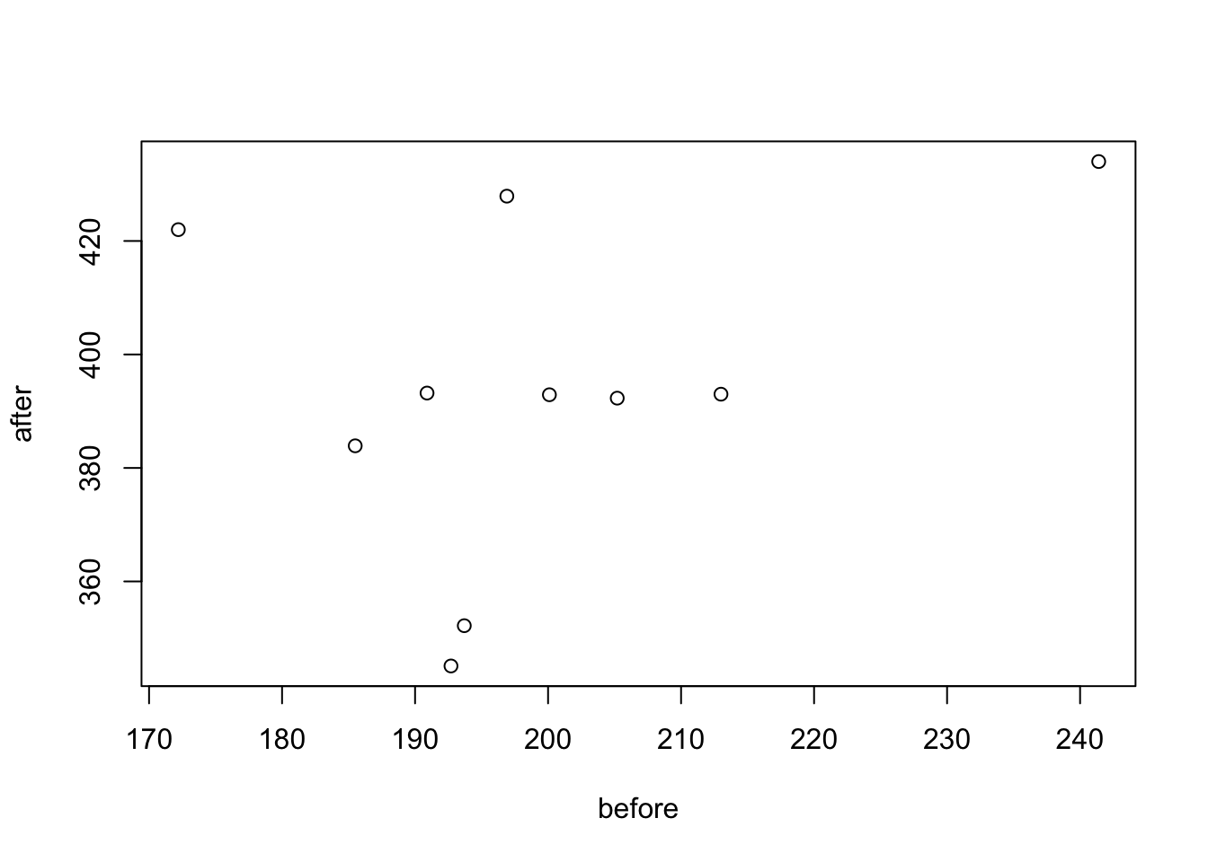
## NULLDue to the small sample size we will want to check again for normality:
# compute the difference between the before and after
d <- with(my_data_paired,
        weight[group == "before"] - weight[group == "after"])

# Shapiro-Wilk normality test for the differences
shapiro.test(d)
##
## Shapiro-Wilk normality test
##
## data: d
## W = 0.94536, p-value = 0.6141Here, as the Shapiro-Wilk normality test p-value is greater than 0.05, we can assume normality.
Let’s so the paired sample t-test:
# Compute t-test
res <- t.test(weight ~ group, data = my_data_paired, paired = TRUE)
res
##
## Paired t-test
##
## data: weight by group
## t = 20.883, df = 9, p-value = 6.2e-09
## alternative hypothesis: true difference in means is not equal to 0
## 95 percent confidence interval:
## 173.4219 215.5581
## sample estimates:
## mean of the differences
## 194.49So the conclusion here is that the p-value of the test is less than the significance level alpha = 0.05, so we can then reject null hypothesis and conclude that the average weight of the mice before treatment is significantly different from the average weight after treatment.
Please also note: if your data are not normally distributed, there are non-parametric tests that you can use instead. For independent t-tests we can use the Mann-Whitney test, which is the wilcox.test() function and for paired t-tests we can use Wilcoxon Rank tests, by using the wilcox.test() function with the paired = TRUE command.