Chapter 11 Applied Data Analytics: More Advanced Topic Modelling
As I had mentioned earlier in the textbook, I wanted to also provide real-life examples using real and noisy data (that sometimes makes you want to cry and reconsider why we wanted to do this work in the first place!) – I’m kidding, although, the more you get into data science, you will encounter projects, data, or types of analysis that test your resilience!
Here, we will look at another way to approach topic modelling. The entire concept is the same as had been shown earlier in the textbook, but we will be using a new package: text2vec and LDAvis. text2vec is an R package that provides a pretty efficient way of doing NLP in R. They have a nice website that shows you everything this package can do here (https://text2vec.org/topic_modeling.html). We are only focusing on Topic Modelling.
All right, let’s get started…
library('dplyr')
library('text2vec')
library('data.table')
library('readr')
library('SnowballC')
So we’ve loaded some packages to get us started. I am using a dataset that contains social media posts from extreme right-wing social media sites. If you’re interested in knowing more, please drop me an email with your questions. Of course, due to the nature of the data… I will NOT be showing any dataviz showing the topics, however, when the final article is out on this, I will create a link to it so you can see them there.
We will read in our data for the analysis…
## Warning: Missing column names filled in: 'X1' [1]##
## ── Column specification ─────────────────────────────────────────────────────────────────────────────────────────────────────────────────────────
## cols(
## X1 = col_double(),
## PPT_ID = col_double(),
## platform = col_character(),
## prosecuted = col_double(),
## arrested = col_character(),
## username = col_character(),
## date = col_character(),
## server = col_character(),
## message = col_character(),
## links = col_double(),
## questionmarks = col_double(),
## exclaimation = col_double(),
## all_punc = col_double(),
## word_count = col_double()
## )##
## ── Column specification ─────────────────────────────────────────────────────────────────────────────────────────────────────────────────────────
## cols(
## X1 = col_character()
## )# This data has lots of columns, but we are only interested the column 'message' here,
#as we need the content to then create our topic models...
# Our first step is to clean the data up a little bit...
#going to get rid of abbreviations in text, as shown in the function:
fix.contractions <- function(doc) {
doc <- gsub("won't", "will not", doc)
doc <- gsub("can't", "can not", doc)
doc <- gsub("n't", " not", doc)
doc <- gsub("'ll", " will", doc)
doc <- gsub("'re", " are", doc)
doc <- gsub("'ve", " have", doc)
doc <- gsub("'m", " am", doc)
doc <- gsub("'d", " would", doc)
doc <- gsub("'s", "", doc)
doc <- gsub("they'r", "they are", doc)
doc <- gsub("they'd", "they had", doc)
doc <- gsub("they'v", "they have", doc)
return(doc)
}
#then we can apply this to our message column
final_data$message = sapply(final_data$message, fix.contractions)
# function to remove special characters throughout the text - so this will be a nicer/easier base to tokenise and analyse
removeSpecialChars <- function(x) gsub("[^a-zA-Z0-9 ]", "", x)
removeNumbers <- function(x) gsub('[[:digit:]]+', '', x)
final_data$message = sapply(final_data$message, removeSpecialChars)
final_data$message = sapply(final_data$message, removeNumbers)
# convert everything to lower case
final_data$message <- sapply(final_data$message, tolower)
#this is never perfect (and is not here!) but you need to check things out iteratively
#until you are happy enough with the cleaningOnce we have finished some cleaning (you can always do more, as the above is a very BASIC form of cleaning)… we can get started with preparation for the topic modelling….
11.1 Data Prep
setDT(final_data) #this forces data into a datatable format
setkey(final_data, X1)  #this is setting an ID column
First, we need to create tokens from our messages… we can also use in-built functions like ‘tolower’, which I have shown here (not necessary as this was already done before). We can also attempt (as these do not always work brilliantly) to stem words (aka, if we had running, ran, and runner, these would all revert to run).
tokens = final_data$message %>%
  tolower %>%
  word_tokenizer #making tokens

tokens = lapply(tokens, SnowballC::wordStem, language="en") #stemming words to help with duplication

it = itoken(tokens, ids = final_data$X1, progressbar = T) #iterating over tokens to build a vocab (see below)
While also loading the dataset, I have also loaded in a smaller csv file of a collection of stop words that I have collected. You can find these online, which I did, and I added my own words, too. This is speciifc to this dataset, as of course, when doing topic modelling we need to remove any words that may be irrelevant and actually just add noise into the topics. One thing to notice is that file formats (and sometimes the langauges themselves like R or python) cannot handle all characters, especially non-ascii ones… so I have a copied list I also put into my stop words based on doing this coding iteratively to remove nonsense characters that add noise to my topic models…
#sorting out stop words (manual and list)
#the stop words list was imported already... and we are making this a vector so then we can add additional
#words and characters to remove
stop_list = as.vector(stop_words[[1]])
#additional characters to manually remove
remove = c("ª",
           "á",
           "å",
           "ä",
           "ç",
           "æ",
           "é",
           "ê",
           "ë",
           "ñ",
           "º",
           "ô",
           "ø",
           "òö",
           "tt",
           "û",
           "ü",
           "µ",
           "ω",
           'ï',
           'ïë',
           'u',
           'ïê',
           'ñì',
           'äî',
           'îå',
           "I'm",
           'im',
           "Im",
           "ð",
           "â",
           "ã",
           "i've",
           "you're",
           "don't",
           "ð_ð",
           "ã_ã",
           "NA",
           'yea',
           'yeah',
           'gonna',
           'dont',
           'oh',
           'org',
           'name',
           'lol',
           'guy',
           'guys',
           'literally',
           'am',
           'actually',
           'getting',
           'lot',
           'little',
           'probably',
           'yes',
           '√§√',
           ',Äç',
           'äù',
           'äì',
           'äôs',
           'äôt',
           '01',
           '02',
           '03',
           '04',
           '05',
           '06',
           '07',
           '08',
           '09')

stop_list = c(stop_list, remove) #merged into one list to remove from model
Next, we create a vocabulary from our tokens, and we can prune this down and remove our stop words. When we prune, this is a manual number we select, and this is based on knowledge of the dataset, so you might need to do this a few times. We have set this to 50, where each term has to appear a minimum of 50 times otherwise it is not included in the vocabulary. Similarly, we ensure that the word is not a obscenely high proportion of the data, so we have set this to 0.1 (aka 10% of the data maximum). We then create a document term matrix (dtm).
v = create_vocabulary(it, stopwords = stop_list) %>%
  prune_vocabulary(term_count_min = 50, doc_proportion_max = 0.1)
vectorizer = vocab_vectorizer(v)


dtm = create_dtm(it, vectorizer, type = "dgTMatrix") #this is just using words (you can use bigrams, for example, too!)
Here, we can proceed with doing our topic modelling! There are a couple ways we can do this…
We can iteratively figure out what the right number of topics is by manually inspecting it…
Or, we can check whats known as topic coherence, which is a data-driven method to see which topics appear to be the most coherent
Both of these are valid topics and often give very different answers.
11.2 Manually testing different numbers of topics
Here we are testing n=4 topics in our dataset.
# note it is really important to set seed here...
#otherwise this will not reproduce each time...!
set.seed(127)
lda_model = LDA$new(n_topics =4, doc_topic_prior = 0.1, topic_word_prior = 0.01)
doc_topic_distr = lda_model$fit_transform(x = dtm, n_iter = 500,
                                          convergence_tol = 0.001, n_check_convergence = 25,
                                          progressbar = T)
Here, we can select a given document (aka a row in the dataset), and see the topics distribtion in each one….
#little data viz...
#this is looking at the proportion of topics in the dataset
barplot(doc_topic_distr[127, ], xlab = "topic",
        ylab = "proportion", ylim = c(0, 1),
        names.arg = 1:ncol(doc_topic_distr))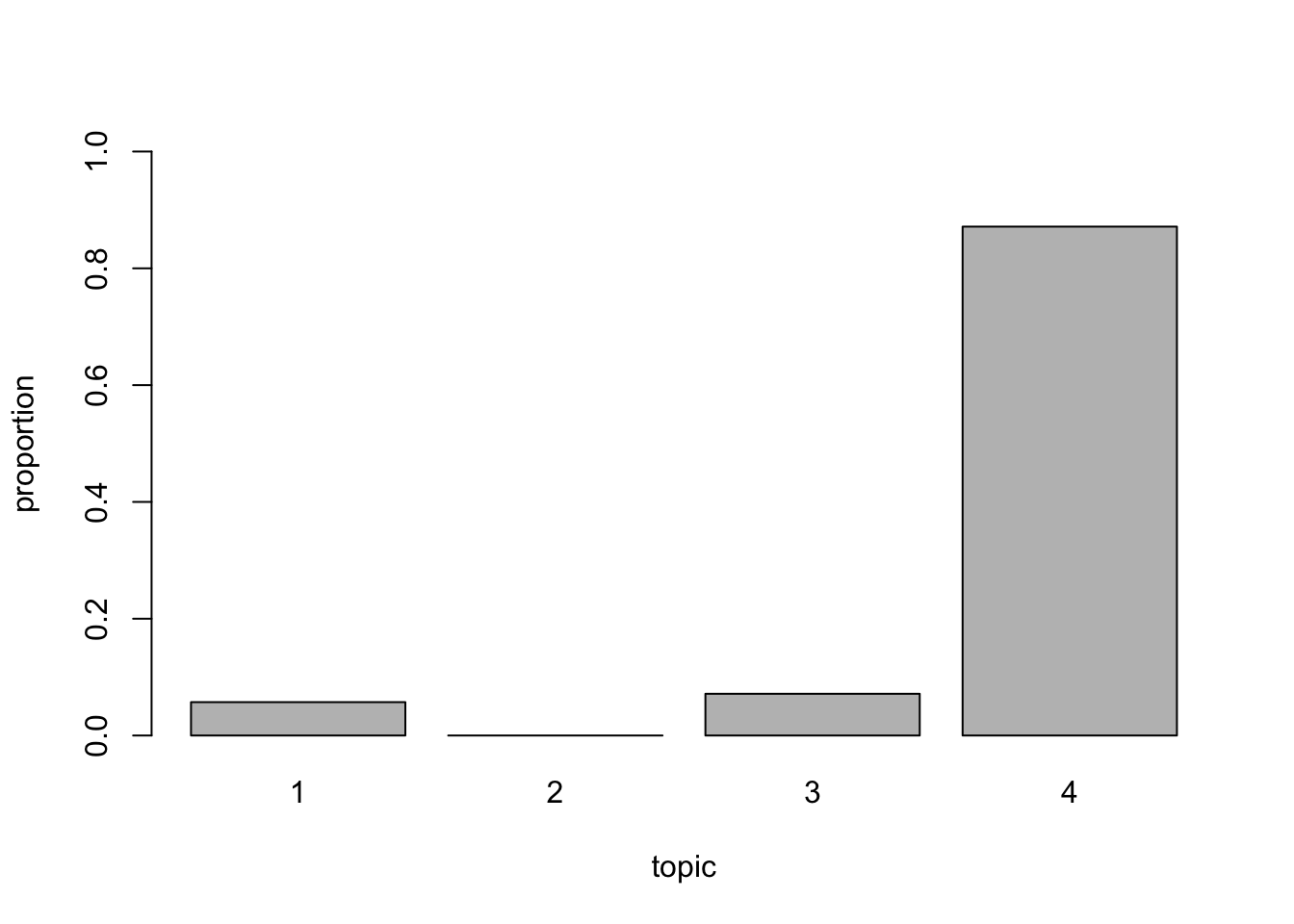
You can of course inspect the topics by calling to look at the top words in each topic:
lda_model$get_top_words(n = 30, topic_number = c(1L,2L,3L,4L), lambda = 0.4)
lda_model$plot()
## Loading required namespace: servr## If the visualization doesn't render, install the servr package
## and re-run serVis:
## install.packages('servr')
## Alternatively, you could configure your default browser to allow
## access to local files as some browsers block this by default#what this does, is it will print the top words (30 of them as we specify) in the console,
#and it will open up an html file, which creates an interactive plot where you can
# see the topics, and change the lambda etc.
#as said above, I have HIDDEN these resutls due to the nature of the data as the
#contents contain some extreme words/views However, it looks something like this:
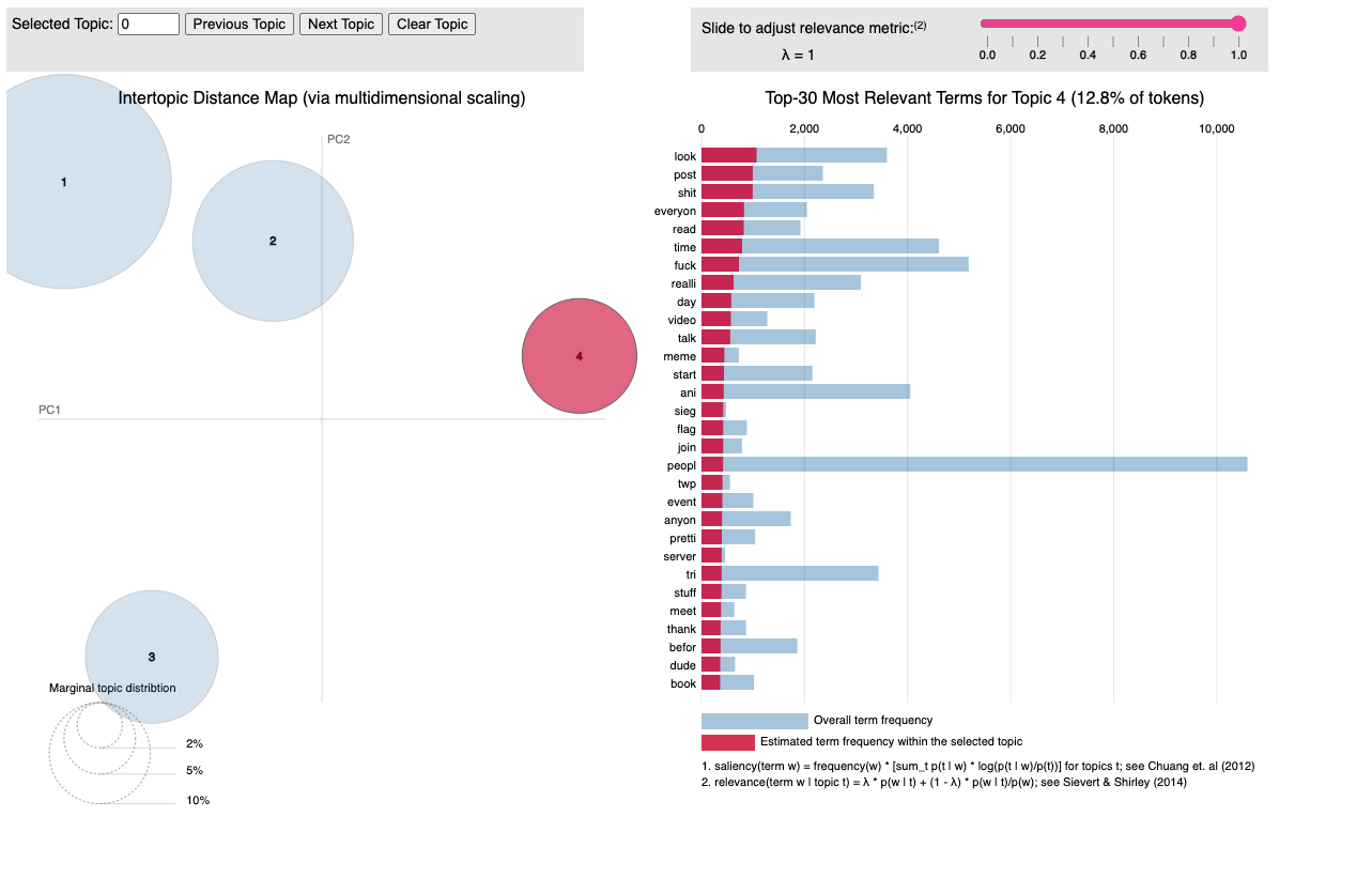
Figure 1. LDA Viz example; note it is actually interactive when run
This provides a nice and interactive way to engage with topics and to clean the content more. This was actually how I found all the additional characters that I needed to remove (in the stop words). So do not worry if you need to run this kind of code again and again – this is all part of the process!
11.3 Topic Coherence Measures
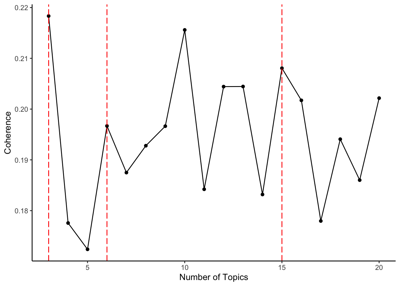
There are a number of different types of topic coherence, but this is one way we used. We were calculating the normalized pointwise mutual information (NPMI), but there are others you can use (e.g., https://search.r-project.org/CRAN/refmans/text2vec/html/coherence.html). Here, in the following code we iterate between 3 to 20 topics by 1 (aka every single number and not skipping any). Note: the code for the coherence metrics was written by Daniel Racek, I tried and panicked, so he helped me figure it out.
Do note, if you run a version of this code (aka please copy cat it if you want to), this will take a while to code as it is literally running a topic model for each of the number of topics between 3 to 20. So give it time and don’t panic!
RcppParallel::setThreadOptions(1)

coh_results = tibble()
for(i in seq(3,20, by = 1)){
  print(i)
  set.seed(127)
  lda_model = LDA$new(n_topics =i, doc_topic_prior = 0.1, topic_word_prior = 0.01)
  doc_topic_distr = lda_model$fit_transform(x = dtm, n_iter = 500,
                                            convergence_tol = 0.001, n_check_convergence = 25,
                                            progressbar = T)

  tcm = create_tcm(it, vectorizer
                   ,skip_grams_window = 110
                   ,weights = rep(1, 110)
                   ,binary_cooccurence = TRUE
  )
  diag(tcm) = attributes(tcm)$word_count
  n_skip_gram_windows = sum(sapply(tokens, function(x) {length(x)}))

  tw = lda_model$get_top_words(n = 50, lambda = 0.4)

  # check coherence
  res = coherence(tw, tcm, metrics = "mean_npmi_cosim2", n_doc_tcm = n_skip_gram_windows)


  coh_results = bind_rows(coh_results, tibble("topic_n" = i, "coh" =  mean(res)))
}

#here we are creating a plot at the most coherent topics... (we know it is 3, 6, 15 based on the above and the plot)

library('ggplot2')
library('ggthemes')
ggplot(data = coh_results) +
  geom_point(aes(topic_n, coh)) +
  geom_line(aes(topic_n, coh)) +
  geom_vline(xintercept=c(3,6,15), color='red',linetype = "longdash")+
  xlab("Number of Topics") +
  ylab("Coherence")+
  theme_classic()