Overlay analyses
library(dplyr)
library(sf)
library(tmap)
library(tmaptools)
library(ggplot2)
library(gridExtra)
library(grid)
Load data
Biophisical data
Load prepared and clipped biophysical layers.
# UPLVI
load("1_data/manual/UPLVI_clip.rData")

# vegetation derived from canopy raster
load("1_data/manual/can_poly_clip.rData")

# bridges
load("1_data/manual/bridges_clip.rData")

# picnic sites
load("1_data/manual/picnic_clip.rData")

# playgrounds
load("1_data/manual/playgrounds_clip.rData")

# sports fields
load("1_data/manual/sports_fields_clip.rData")

# stairs
load("1_data/manual/stairs_clip.rData")

# trails
load("1_data/manual/trails_clip.rData")

# roads
load("1_data/manual/road_ws_clip.rData")

# curbs
load("1_data/manual/curbs_clip.rData")
Pinch-points
Load buffered pinch-point polygons
Base layers
Load baselayers to be used for visualization maps.
Intersect polygon layers with pinch points
Intersect the spatial covariates with the pinch-point buffer polygons. Then calculate the area of the all of the new clipped polygons generated.
# list objects to individually intersect by the pinchpoints
x<-list(UPLVI_clip, can_poly_clip, picnic_clip, playgrounds_clip, sports_fields_clip)
names(x)<-c("UPLVI_int", "can_poly_int", "picnic_int", "playgrounds_int", "sports_fields_int")

# calculate the area of the buffered pinchpoints
pp_s_clip_clus_buf_ext$buf_area<-st_area(pp_s_clip_clus_buf_ext)


#apply the following to all the layers
nx<-lapply(x, function(x)
  {
  a<-st_intersection(x, pp_s_clip_clus_buf_ext)
  cbind(a, "int_area"=st_area(a)) #calculate area of new clipped polygons
  })

#save new intersection objects
lapply(names(nx),function(x)
  { assign(x,nx[[x]])
  save(list=x, file=paste("3_pipeline/tmp/", x, ".rdata", sep = ""))
  })

# put intersection objects into the global environment
list2env(nx, .GlobalEnv)


##################################################################
# generate plots to illustrate
m1<-
  tm_shape(UPLVI_clip)+
    tm_fill(col="LANDCLAS1", palette = "Dark2", contrast = c(0.26, 1),alpha = .3, legend.show = FALSE) +
  tm_shape(v_road_clip)+tm_lines(col="white", lwd=1)+
  #tm_layout(bg.col="#d9d9d9")+
  tm_shape(nscr)+
    tm_fill(col="white", alpha=.7)+
    tm_borders(col = "#636363")+
    #tm_borders(col = "#636363")
  tm_shape(UPLVI_int)+
    tm_fill(col="LANDCLAS1", palette = "Dark2", contrast = c(0.26, 1),alpha = 1, title="Land Classification", labels = c("Developed","Modified", "Natural", "Naturally Wooded", "Naturally Non-Wooded"))+
  tm_shape(pp_s_clip_clus_buf_ext)+
    tm_borders(col = "#636363",
               lwd= .5)+
  tm_layout(legend.outside = FALSE, legend.text.size = .8, legend.bg.color="white", legend.frame=TRUE,legend.title.size=1, legend.frame.lwd=.8)
m1

tmap_save(m1, "4_output/maps/UPLVI_int_map.png", outer.margins=c(0,0,0,0))

# convert geometry to polygons so can_poly_int plots properly
can_poly_int<-st_collection_extract(can_poly_int, "POLYGON")

m2<-
  tm_shape(v_road_clip)+tm_lines(col="white")+
  tm_layout(bg.col="#d9d9d9")+
  tm_shape(nscr)+
    tm_fill(col="white", alpha=.7)+
    tm_borders(col = "#636363")+
  tm_shape(can_poly_clip)+
    tm_fill(col="Class", palette = "Dark2", contrast = c(0.26, 1),alpha = .3, legend.show = FALSE)+
  tm_shape(nscr)+
    tm_fill(col="white", alpha=.7)+
    tm_borders(col = "#636363")+
    #tm_borders(col = "#636363")
  tm_shape(can_poly_int)+
    tm_fill(col="Class", palette = "Dark2", contrast = c(0.26, 1),alpha = 1, title="Vegetation class")+
  tm_shape(pp_s_clip_clus_buf_ext)+
    tm_borders(col = "#636363",
               lwd= .5)+
  tm_layout(legend.outside = FALSE, legend.text.size = .8, legend.bg.color="white", legend.frame=TRUE,legend.title.size=1, legend.frame.lwd=.8)
m2

tmap_save(m2, "4_output/maps/can_poly_int_map.png", outer.margins=c(0,0,0,0))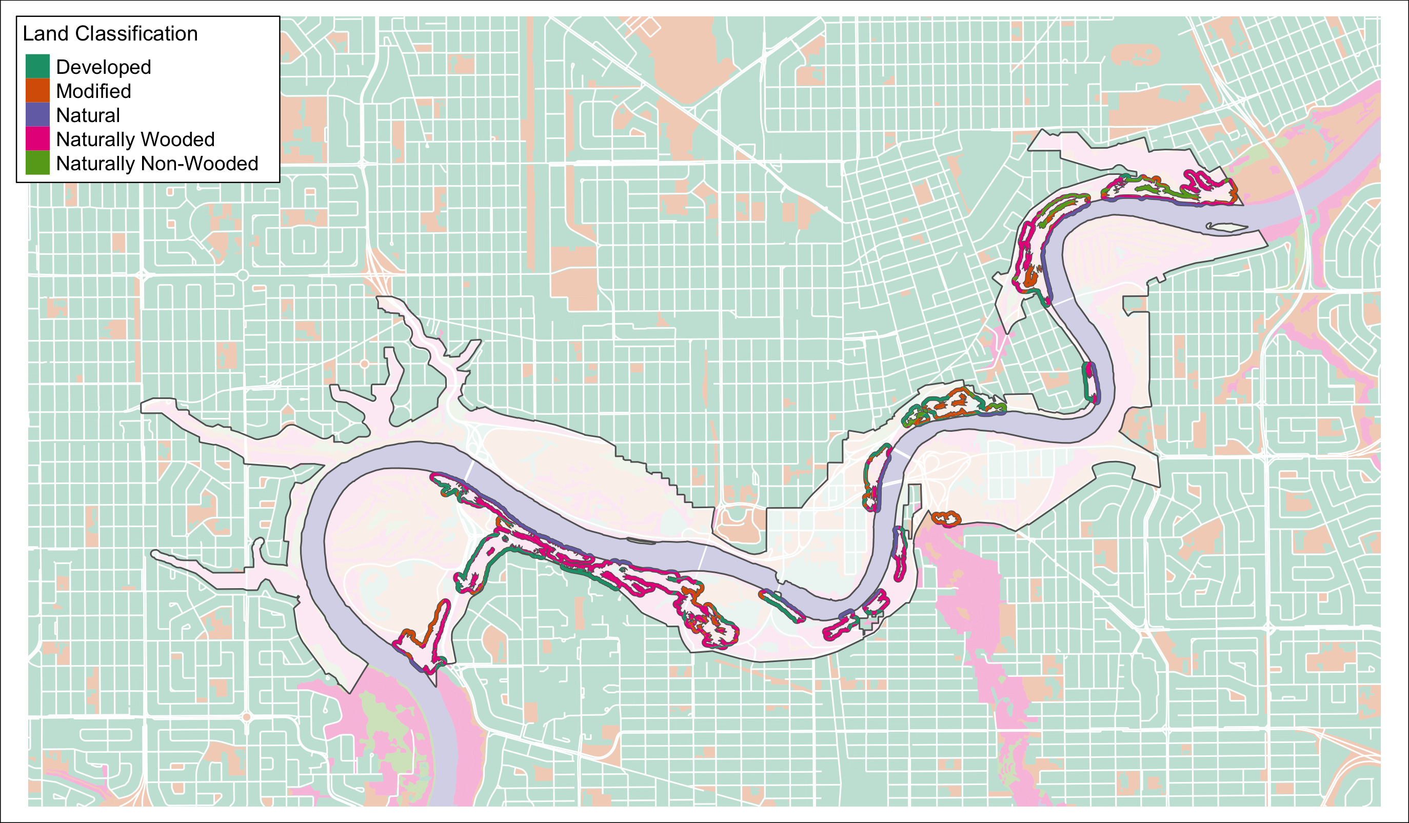
Figure 3.1: UPLVI clipped to pinchpoint buffers.

Figure 3.2: Canopy polygons clipped to pinchpoint buffers.
Calculate proportion of cover
From canopy polygons
load("3_pipeline/tmp/can_poly_int.rData")

# convert geometry to polygons so can_poly_int plots properly
can_poly_int<-st_collection_extract(can_poly_int, "POLYGON")

x<-can_poly_int
xSum<-as.data.frame(x) %>%
  group_by(group, Class)%>%
  summarize(mean=mean(area))%>%
  mutate(proportion=as.numeric(mean/sum(mean)))

xSum<-inner_join(pp_s_clip_clus_buf, xSum, by=c("group"="group"))
xSum$group<-as.factor(xSum$group)


######################### Plot with barplots as icons   ##############################

# get color pallette
origin_cols<- c("Grass"= "#1b9e77", "Shrub-Dec"="#d95f02", "Tree-Con"="#7570b3", "Tree-Dec"="#e7298a")

# create bar plots in ggplot convert to grob objects which will be plotted in tmap.
grobs <- lapply(split(xSum, factor(xSum$group)), function(x) {
ggplotGrob(ggplot(x, aes("", y=proportion, fill=Class, label = group)) +
    geom_bar(width=1, stat="identity", colour="black", lwd=.2) +
    scale_y_continuous(expand=c(0,0)) +
    scale_fill_manual(values=origin_cols) +
    theme_ps(plot.axes = FALSE)
)
}
)


m3<-
  tm_shape(v_road_clip)+tm_lines(col="white")+
  tm_layout(bg.col="#d9d9d9")+
  tm_shape(nscr)+
    tm_fill(col="white", alpha=.4)+
    tm_borders(col = "#636363")+
  tm_shape(xSum)  +
    tm_fill(col="MAP_COLORS", palette = "Dark2", alpha=.6)+
    tm_borders(alpha=1)+
    tm_symbols(shape="group",
        shapes=grobs,
        border.lwd = 0,
          #sizes.legend=c(.5, 1,3)*1e6,
          scale=.6,
        clustering=TRUE,
          legend.shape.show = FALSE,
          legend.size.is.portrait = TRUE,
          # shapes.legend = 22,
          # group = "Charts",
        #id = "group",
        breaks = "fixed",
      labels = "Class")+
#         popup.vars = c("NVE", "VEG"))
  #tm_shape(pp_s_clip_clus_buf)+

  #tm_text(text = "group")+
tm_add_legend(type="fill",
          group = "Charts",
          labels = c("Grass", "Shrub-Dec", "Tree-Con", "Tree-Dec"),
          col=c("#1b9e77", "#d95f02", "#7570b3", "#e7298a"),
          title="Class")+
tm_layout(legend.outside = FALSE, legend.text.size = .8, legend.bg.color="white", legend.frame=TRUE, legend.frame.lwd=.8,
          legend.position=c("left", "top"))
m3

tmap_save(m3, "4_output/maps/summary/can_poly_sum_map.png", outer.margins=c(0,0,0,0))

############################# barplots under the map ############################

m4<-
  tm_shape(v_road_clip)+tm_lines(col="white")+
  tm_layout(bg.col="#d9d9d9")+
  tm_shape(nscr)+
    tm_fill(col="white", alpha=.4)+
    tm_borders(col = "#636363")+
  tm_shape(pp_s_clip_clus)  +
    tm_fill(col="MAP_COLORS", palette = "Dark2", alpha=.8)+
    tm_borders(alpha=1)+
   tm_shape(xSum)+
    tm_text(text = "group",
          col="black",
          size = 1.5)+
          # bg.color="white",
          # bg.alpha=.1)+
 # tm_shape(pp_s_clip_clus)  +
 #   tm_polygons()+
 #     tm_borders(
 #       col = "red",
 #       )+
tm_add_legend(type="fill",
          group = "Charts",
          labels = c("Grass", "Shrub-Dec", "Tree-Con", "Tree-Dec"),
          col=c("#1b9e77", "#d95f02", "#7570b3", "#e7298a"),
          title="Class")+
tm_layout(legend.show=FALSE, legend.outside = FALSE, legend.text.size = .8, legend.bg.color="white", legend.frame=TRUE, legend.frame.lwd=.8,
          legend.position=c("left", "bottom"))

m4

t_grob<-tmap_grob(m4)

# convert map to grob object
g1<-arrangeGrob(t_grob)

g2<-xSum%>%
    ggplot(aes(x = group, y = proportion, fill=Class, label = group)) +
    geom_bar(width=.8, stat="identity", colour="black", lwd=.2) +
    labs(x="pinch-point", y="% cover")+
    scale_y_continuous(labels=scales::percent) +
    theme(panel.spacing = unit(1, "lines"),
          panel.background = element_blank(),
          axis.ticks=element_blank())

 lay2 <- rbind(c(1),
              c(1),
              c(1),
              c(2))

g3<-arrangeGrob(g1, g2, layout_matrix =lay2)
ggsave("4_output/maps/summary/can_poly_sum_map_2.png", g3, width=11, height=9)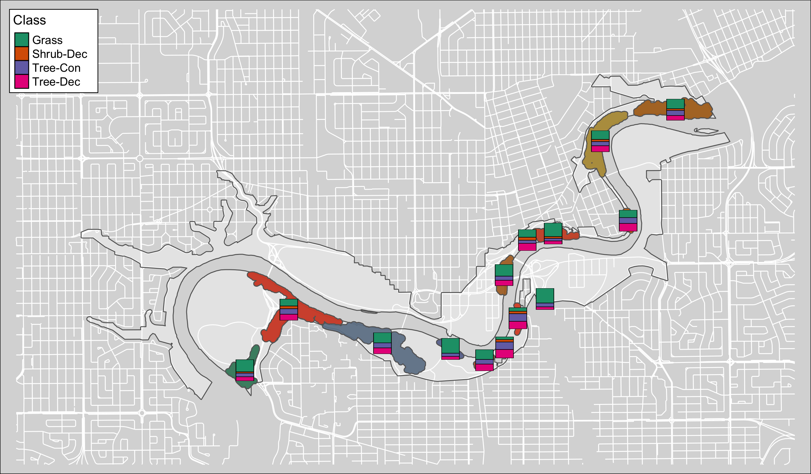
Figure 3.3: Canopy poly class map #1.
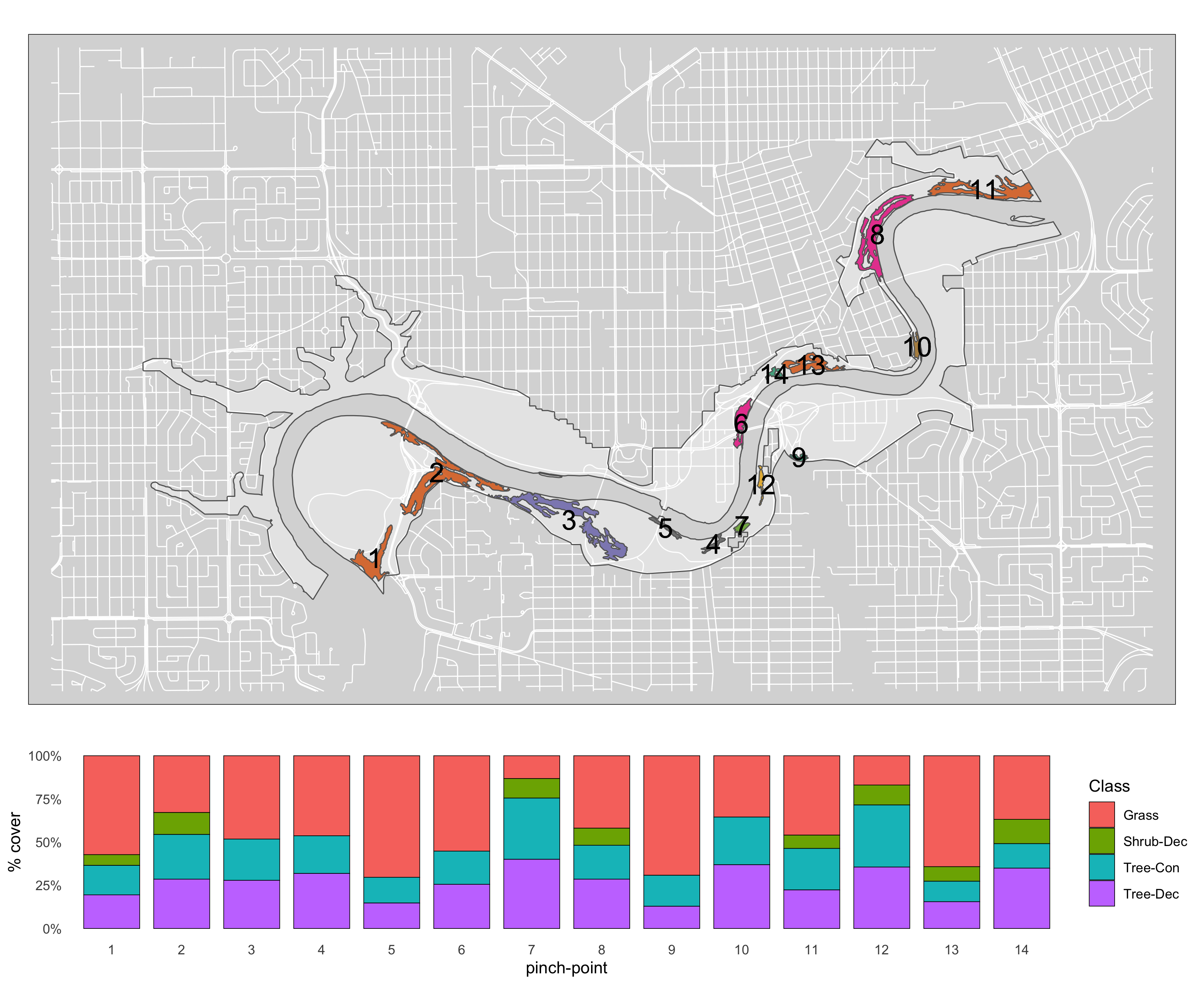
Figure 3.4: Canopy poly class map #2.
From UPLVI
`Extract STYPE values for each polygon. Include area and percentage per STYPE
load("3_pipeline/tmp/UPLVI_int.rData")

# create a new dataframe with only necessary columns

TYPE<-as.data.frame(UPLVI_int[c(1,61:62, 4:7, 23:26, 42:45, 63:64)])

#seperate STYPPE ranks into seperate dataframes
a<-TYPE[c(1:3, 4:7, 16:17)]
b<-TYPE[c(1:3, 8:11, 16:17)]
c<-TYPE[c(1:3, 12:15, 16:17)]

# rename columns so they are constant
b<-setNames(b, names(a))
c<-setNames(c, names(a))

#rbind dataframes together
abc<-rbind(a, b, c)

# create a column with just rank number of STYPES
s_rank<-gather(TYPE, "STYPE_rank", "STYPE", c(4,8,12))

# add the rank column
abcf<-cbind(abc, s_rank$STYPE_rank)

#reorder columns
abcf<-abcf[c(1:3, 8, 4:7)]

# rename columns
colnames(abcf)[c(4:7, 10)]<-c("PRIMECLAS", "LANDCLAS", "STYPE", "STYPEPER", "s_rank")

# approximate area of each STYPE class/ polygon by multipltying the percentage by polygon area. Creates a new column
# calculate proportion of each polygon covered by STYPE class

# here is a way to loop through a bunch of column
v<- abcf[4:6] #select the columns that you want to use for landcover data
vnames <- colnames(v)
a <- list()
j = 1
for (i in v) {
  a[[j]] <- abcf %>%
    group_by(POLY_NUM, ID, {{i}})%>%
    mutate(s_area=as.numeric((STYPEPER*.1)*int_area))%>%
    group_by(ID, {{i}})%>%
    mutate(t_area=sum(s_area))%>%
    select(-s_rank, -STYPEPER, -s_area, -int_area, -POLY_NUM, -group, -LANDCLAS,-STYPE, -PRIMECLAS)%>%
    distinct()%>%
    na.omit()%>%
    mutate(t_proportion=as.numeric(t_area/buf_area))%>%
    select(-buf_area)%>%
    arrange(ID)
  names(a)[j]=vnames[j] #name list item
  colnames(a[[j]])[2]<- vnames[j] # name variable column
  #a[[j]]$vnames = vnames[j]
  j = j + 1
}
a

UPLVI_class_cov<-a

save(UPLVI_class_cov, file="3_pipeline/store/UPLVI_class_cov.rData")


# #non loop, one variable at a time
# STYPE_area<-
#   abcf %>%
#   group_by(POLY_NUM, ID, STYPE)%>%
#   mutate(s_area=as.numeric((STYPEPER*.1)*int_area))%>%
#   group_by(ID, STYPE)%>%
#   mutate(t_area=sum(s_area))%>%
#   select(-s_rank, -STYPEPER, -s_area, -int_area, -POLY_NUM, -group)%>%
#   distinct()%>%
#   na.omit()%>%
#   mutate(t_proportion=as.numeric(t_area/buf_area))%>%
#   select(-buf_area)%>%
#   arrange(ID)
#   #group_by(ID)%>%
#   #mutate(t_proportion_sum=sum(t_proportion))
#
# save(STYPE_area, file="3_pipeline/store/STYPE_area.rData")


######################################################################

# # function that that calculates proportions
# x_summary<-function(x) {
#   df %>%
#   group_by(ID, {{x}})%>%
#   summarize(mean=mean(area))%>%
#   mutate(proportion=as.numeric(mean/sum(mean)))
# }
#
# # here is a way to loop through a bunch of column
# v<- df[4:6] #select the columns that you want to use for landcover data
# vnames <- colnames(v)
# a <- list()
# j = 1
# for (i in v) {
#   a[[j]] <- df %>%
#     group_by(ID, {{i}})%>%
#     summarize(mean=mean(area))%>%
#     mutate(proportion=as.numeric(mean/sum(mean)))
#   names(a)[j]=vnames[j] #name list item
#   colnames(a[[j]])[2]<- vnames[j] # name variable column
#   a[[j]]$vnames = vnames[j]
#   j = j + 1
# }
# a| ID | STYPE | t_area | t_proportion |
|---|---|---|---|
| 1 | FT | 3.057096e+04 | 0.4896048 |
| 1 | ERC | 2.049324e+03 | 0.0328207 |
| 1 | MG | 1.761568e+04 | 0.2821215 |
| 1 | AIH | 1.261320e+03 | 0.0202005 |
| 1 | NW | 6.205953e+03 | 0.0993906 |
| 1 | CS | 2.803509e+02 | 0.0044899 |
| 1 | TT | 4.456476e+03 | 0.0713721 |
| 2 | FT | 7.727468e+04 | 0.4196452 |
| 2 | ECS | 2.534530e+03 | 0.0137639 |
| 2 | ERC | 1.755813e+04 | 0.0953506 |
| 2 | MG | 1.272672e+04 | 0.0691133 |
| 2 | AIH | 1.648611e+04 | 0.0895289 |
| 2 | TT | 3.343063e+03 | 0.0181547 |
| 2 | AW | 2.020008e+03 | 0.0109698 |
| 2 | BPC | 7.146034e+03 | 0.0388070 |
| 2 | NW | 3.563878e+04 | 0.1935387 |
| 2 | NG | 5.162899e+02 | 0.0028037 |
| 2 | MS | 8.898580e+03 | 0.0483243 |
| 3 | FT | 1.062281e+05 | 0.5915171 |
| 3 | MG | 2.816398e+04 | 0.1568274 |
| 3 | AIH | 5.062579e+03 | 0.0281903 |
| 3 | BPC | 1.087910e+04 | 0.0605788 |
| 3 | ECS | 1.434101e+04 | 0.0798560 |
| 3 | NW | 7.621390e+03 | 0.0424387 |
| 3 | ERC | 3.585252e+03 | 0.0199640 |
| 3 | MS | 3.704453e+03 | 0.0206278 |
| 4 | FT | 1.343942e+04 | 0.4978438 |
| 4 | ERC | 3.328728e+03 | 0.1233079 |
| 4 | EMS | 9.406371e+02 | 0.0348445 |
| 4 | NW | 3.580878e+03 | 0.1326484 |
| 4 | MG | 4.184974e+03 | 0.1550263 |
| 4 | TT | 3.698587e+02 | 0.0137009 |
| 4 | OS | 1.045152e+02 | 0.0038716 |
| 4 | AIH | 1.046244e+03 | 0.0387566 |
| 5 | BPC | 4.213787e+02 | 0.0155097 |
| 5 | FT | 4.146730e+03 | 0.1526290 |
| 5 | AIH | 4.356227e+02 | 0.0160340 |
| 5 | CDS | 1.246528e+04 | 0.4588106 |
| 5 | MG | 1.321398e+03 | 0.0486368 |
| 5 | NW | 6.775280e+03 | 0.2493783 |
| 5 | MS | 1.036682e+03 | 0.0381573 |
| 5 | MT | 5.663136e+02 | 0.0208443 |
| 6 | MG | 6.559745e+03 | 0.1468837 |
| 6 | ERC | 1.934790e+03 | 0.0433232 |
| 6 | BPC | 6.153364e+02 | 0.0137784 |
| 6 | FT | 1.130992e+04 | 0.2532480 |
| 6 | AIH | 9.348889e+03 | 0.2093372 |
| 6 | NW | 1.259376e+04 | 0.2819954 |
| 6 | TT | 1.079156e+03 | 0.0241641 |
| 6 | MT | 1.217867e+03 | 0.0272701 |
| 7 | FT | 1.192429e+04 | 0.6417167 |
| 7 | ERC | 2.684325e+03 | 0.1444594 |
| 7 | EMS | 3.307491e+03 | 0.1779956 |
| 7 | TT | 2.982583e+02 | 0.0160510 |
| 7 | OS | 3.674990e+02 | 0.0197773 |
| 8 | ERC | 7.351254e+03 | 0.0603288 |
| 8 | CS | 2.472962e+04 | 0.2029462 |
| 8 | FT | 3.403659e+04 | 0.2793249 |
| 8 | HG | 8.267949e+03 | 0.0678518 |
| 8 | MG | 1.440160e+04 | 0.1181883 |
| 8 | AIH | 6.208355e+02 | 0.0050950 |
| 8 | NW | 2.249149e+04 | 0.1845788 |
| 8 | MS | 2.385802e+03 | 0.0195793 |
| 8 | MT | 2.058090e+03 | 0.0168899 |
| 8 | TT | 4.112830e+03 | 0.0337524 |
| 8 | EMS | 6.052187e+02 | 0.0049668 |
| 8 | NMS | 7.917676e+02 | 0.0064977 |
| 9 | FT | 2.287642e+03 | 0.1338340 |
| 9 | NG | 6.300555e+02 | 0.0368602 |
| 9 | TT | 3.066682e+03 | 0.1794102 |
| 9 | MG | 7.035434e+03 | 0.4115942 |
| 9 | AIH | 4.068857e+03 | 0.2380405 |
| 9 | MT | 4.461994e+00 | 0.0002610 |
| 10 | AF | 1.778758e+02 | 0.0064783 |
| 10 | ERC | 1.064639e+04 | 0.3877424 |
| 10 | FT | 7.492008e+03 | 0.2728596 |
| 10 | NW | 9.141101e+03 | 0.3329197 |
| 11 | MG | 1.120536e+04 | 0.0981622 |
| 11 | HG | 1.142510e+04 | 0.1000872 |
| 11 | FT | 4.255131e+04 | 0.3727621 |
| 11 | CS | 1.465992e+04 | 0.1284253 |
| 11 | ERC | 3.014000e+03 | 0.0264035 |
| 11 | NW | 1.655449e+04 | 0.1450222 |
| 11 | TT | 2.943175e+03 | 0.0257831 |
| 11 | EMS | 5.248841e+03 | 0.0459814 |
| 11 | MS | 3.353393e+03 | 0.0293767 |
| 11 | NG | 1.381347e+03 | 0.0121010 |
| 11 | MT | 3.619217e+02 | 0.0031705 |
| 11 | NMS | 1.452538e+03 | 0.0127247 |
| 12 | FT | 1.813865e+04 | 0.6180288 |
| 12 | BPC | 2.778148e+03 | 0.0946584 |
| 12 | EMS | 6.107858e+03 | 0.2081099 |
| 12 | ERC | 1.189396e+03 | 0.0405257 |
| 12 | NW | 4.564966e+02 | 0.0155540 |
| 12 | OS | 6.786509e+02 | 0.0231233 |
| 13 | CS | 4.379030e+03 | 0.0726516 |
| 13 | NG | 1.801077e+04 | 0.2988129 |
| 13 | AF | 3.942104e+03 | 0.0654026 |
| 13 | BPC | 9.689234e+03 | 0.1607521 |
| 13 | MG | 4.638828e+03 | 0.0769618 |
| 13 | ERC | 2.169972e+02 | 0.0036002 |
| 13 | NW | 5.144802e+03 | 0.0853564 |
| 13 | AIH | 6.807291e+03 | 0.1129384 |
| 13 | FT | 2.937459e+02 | 0.0048735 |
| 13 | TT | 3.728944e+03 | 0.0618661 |
| 13 | MT | 3.422651e+03 | 0.0567845 |
| 14 | FT | 3.226432e+03 | 0.1414977 |
| 14 | MG | 1.630562e+03 | 0.0715096 |
| 14 | CS | 4.454333e+03 | 0.1953482 |
| 14 | NG | 1.806718e+03 | 0.0792350 |
| 14 | BPC | 2.958360e+03 | 0.1297412 |
| 14 | AIH | 3.621900e+03 | 0.1588412 |
| 14 | ECS | 1.290115e+03 | 0.0565790 |
| 14 | NW | 6.307969e+02 | 0.0276641 |
| 14 | AF | 1.024415e+03 | 0.0449265 |
| 14 | TT | 8.247446e+02 | 0.0361698 |
| 14 | ERC | 8.600767e+02 | 0.0377193 |
| 14 | MT | 4.735583e+02 | 0.0207683 |
Visualize
m5<-
  tm_shape(v_road_clip)+tm_lines(col="white")+
  tm_layout(bg.col="#d9d9d9")+
  tm_shape(nscr)+
    tm_fill(col="white", alpha=.4)+
    tm_borders(col = "#636363")+
  tm_shape(pp_s_clip_clus)  +
    tm_fill(col="MAP_COLORS", palette = "Dark2", alpha=.8)+
    tm_borders(alpha=1)+
   tm_shape(pp_s_clip_clus_buf)+
    tm_text(text = "group",
          col="black",
          size = 1.5)+
          # bg.color="white",
          # bg.alpha=.1)+
 # tm_shape(pp_s_clip_clus)  +
 #   tm_polygons()+
 #     tm_borders(
 #       col = "red",
 #       )+
tm_add_legend(type="fill",
          group = "Charts",
          labels = c("Grass", "Shrub-Dec", "Tree-Con", "Tree-Dec"),
          col=c("#1b9e77", "#d95f02", "#7570b3", "#e7298a"),
          title="Class")+
tm_layout(legend.show=FALSE, legend.outside = FALSE, legend.text.size = .8, legend.bg.color="white", legend.frame=TRUE, legend.frame.lwd=.8,
          legend.position=c("left", "bottom"))

m5

t_grob<-tmap_grob(m5)

# convert map to grob object
g1<-arrangeGrob(t_grob)


g2<-UPLVI_class_cov$PRIMECLAS%>%
    ggplot(aes(x = factor(ID), y = t_proportion, fill=PRIMECLAS, label = ID)) +
    geom_bar(width=.8, stat="identity", colour="black", lwd=.2) +
    labs(x="pinch-point", y="% cover")+
    scale_y_continuous(labels=scales::percent,position = "right") +
    guides(fill=guide_legend(ncol=3))+
    theme(panel.spacing = unit(1, "lines"),
          panel.background = element_blank(),
          axis.title = element_text(colour = "white"),
          axis.ticks=element_blank(),
          #plot.margin=margin(0,0,0,50),
          #legend.key.width=unit(.5,"cm"),
          legend.position = "left")
          #legend.position="left")


g3<-UPLVI_class_cov$LANDCLAS%>%
    ggplot(aes(x = factor(ID), y = t_proportion, fill=LANDCLAS, label = ID)) +
    geom_bar(width=.8, stat="identity", colour="black", lwd=.2) +
    labs(x="pinch-point", y="% cover")+
    scale_y_continuous(labels=scales::percent, position = "right") +
    guides(fill=guide_legend(ncol=3))+
    theme(panel.spacing = unit(1, "lines"),
          panel.background = element_blank(),
          axis.title.x = element_text(colour = "white"),
          axis.ticks=element_blank(),
          #plot.margin=margin(0,0,0,50),
          #legend.key.width=unit(.5,"cm"),
          legend.position = "left")
          #legend.position="left")

g4<-UPLVI_class_cov$STYPE%>%
    ggplot(aes(x = factor(ID), y = t_proportion, fill=STYPE, label = ID)) +
    geom_bar(width=.8, stat="identity", colour="black", lwd=.2) +
    labs(x="pinch-point", y="% cover")+
    scale_y_continuous(labels=scales::percent, position = "right") +
    #scale_x_discrete(labels= as.character(ID), breaks= ID)+
    guides(fill=guide_legend(ncol=3))+
    theme(panel.spacing = unit(1, "lines"),
          panel.background = element_blank(),
          axis.title.y = element_text(colour = "white"),
          axis.ticks=element_blank(),
          #plot.margin=margin(0,0,0,50),
          #legend.key.width=unit(.5,"cm"),
          legend.position = "left")
          #legend.position="bottom")


 lay2 <- rbind(c(1),
              c(1),
              c(1),
              c(2),
              c(3),
              c(4))

g5<-arrangeGrob(g1, g2, g3, g4, layout_matrix =lay2)
ggsave("4_output/maps/summary/UPLVI_class_cov_map.png", g5, width=11, height=14)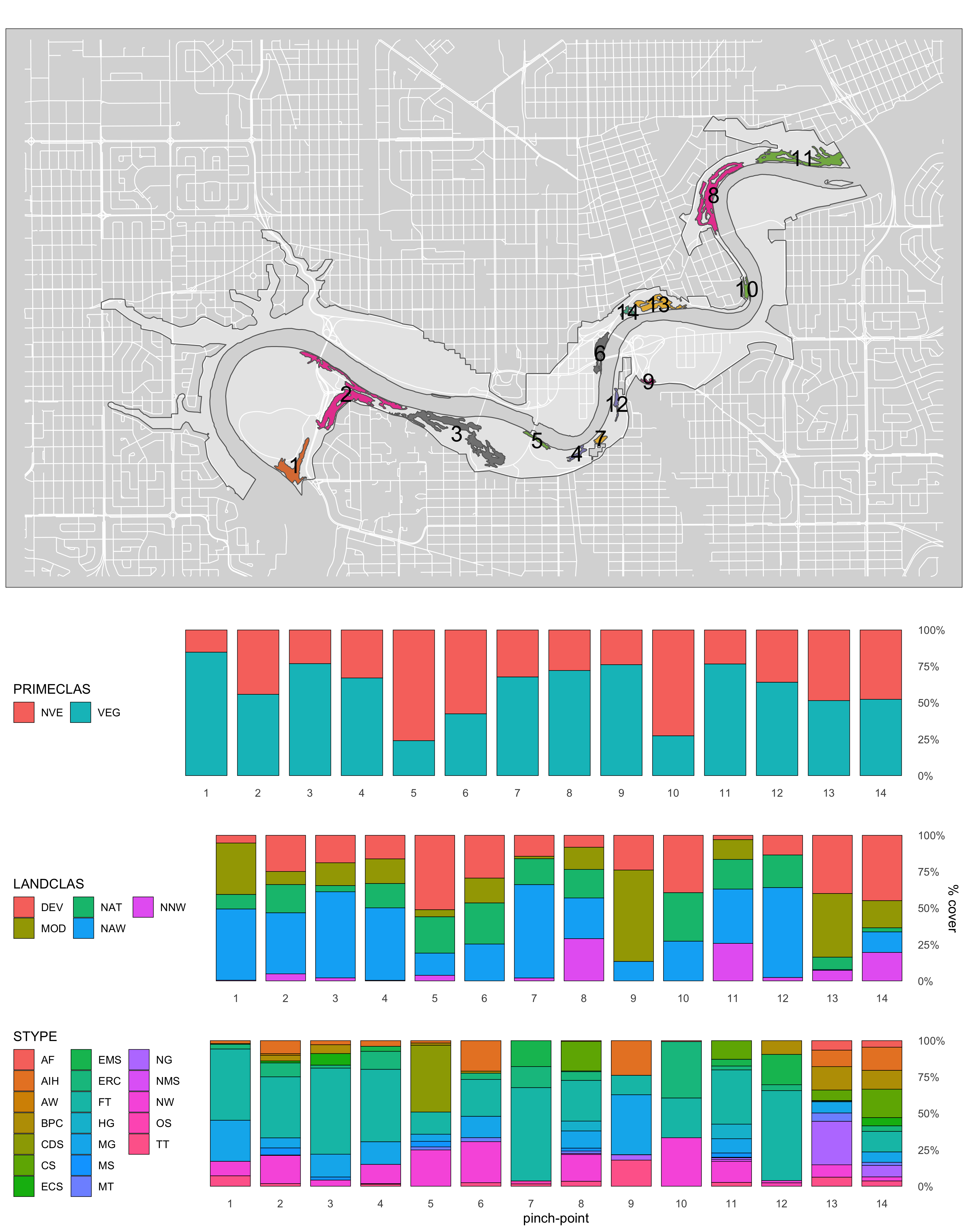
Figure 3.5: Canopy poly class map #2.