第 8 章 模型构建
如何运用光谱实现对目标性状进行预测或者对目标类别进行准确判定,那就需要运用一些模型构建的方法进行自变量和因变量的拟合,这里的因变量就是我们要预测或者判别的目标性状和类别,自变量就是我们的光谱数据了,光谱数据大多用来做判别分析或者回归预测,用来判别或者预测的模型,目前主要包括机器学习模型,机器学习主要包括监督学习、无监督学习以及强化学习三种,我们可以看看维基百科上是怎么说的,
机器学习是人工智能的一个分支。人工智能的研究历史有着一条从以“推理”为重点,到以“知识”为重点,再到以“学习”为重点的自然、清晰的脉络。显然,机器学习是实现人工智能的一个途径,即以机器学习为手段解决人工智能中的问题。机器学习在近30多年已发展为一门多领域交叉学科,涉及概率论、统计学、逼近论、凸分析、计算复杂性理论等多门学科。机器学习理论主要是设计和分析一些让计算机可以自动“学习”的算法。机器学习算法是一类从数据中自动分析获得规律,并利用规律对未知数据进行预测的算法。因为学习算法中涉及了大量的统计学理论,机器学习与推断统计学联系尤为密切,也被称为统计学习理论。算法设计方面,机器学习理论关注可以实现的,行之有效的学习算法。很多推论问题属于无程序可循难度,所以部分的机器学习研究是开发容易处理的近似算法.
接下来我们将从这两大部分进行深入讨论。即判别模型和预测模型,判别模型通常用来做类别判别,而预测模型通常是回归模型,用来做数据的预测反演的。
8.1 判别模型
在机器学习领域判别模型是一种对未知数据 y 与已知数据x之间关系进行建模的方法。判别模型是一种基于概率理论的方法。已知输入变量 x ,判别模型通过构建条件概率分布预测y。常见的判别分析模型有
支持向量机模型(Support Vector Machine, SVM),随机森林模型(Random Forests,RF),决策树(Decision Tree,DT),
人工神经网络(Artificial Neural Network,ANN),偏最小二乘判别法(PLSDA)。这些模型在R语言中,有很多包可以实现判别模型构建,而且代码会很简单,十分容易理解。这里我们挑
选原始光谱进行构建判别分析模型,并对比其模型准确率,给大家一个直观的感受,这些数据我是分了4个不同种源的笋类,因此我想构建一个可以准确鉴别这四种种源竹笋的判别模型。我将从SVM、RF、DT、ANN,PLSDA等五种判别模型方法进行演示。
8.1.1 SVM模型
维基百科上是这样解释SVM算法的:
>SVM是在分类与回归分析中分析数据的监督式学习模型与相关的学习算法。给定一组训练实例,每个训练实例被标记为属于两个类别中的一个或另一个,SVM训练算法创建一个将新的实例分配给两个类别之一的模型,使其成为非概率二元线性分类器。SVM模型是将实例表示为空间中的点,这样映射就使得单独类别的实例被尽可能宽的明显的间隔分开。然后,将新的实例映射到同一空间,并基于它们落在间隔的哪一侧来预测所属类别。
SVM模型。这里我们用e1071安装包来实现:
首先我们进行数据规整,我们将光谱数据单独命名,然后再从总数据里面提取y值,也就是我们的因变量,然后合成一个新的用来运算的数据集,结果如下
library(e1071)
library(prospectr)
#提取光谱数据和其已知种源信息
nir <- as.matrix(spec[,-c(1:2,238:258)])
orig <- spec$typee
#用这两个指标构建一个新的dataframe 数据
data_new <- data.frame(y=orig,x=nir)
head(data_new)[1:5,1:10]#为防止篇幅过长,这里只显示前5行,10列。
## y x.976.3 x.981.7 x.987.2 x.992.7 x.998.3 x.1004 x.1009.7 x.1015.5 x.1021.3
## 1 BJ 0.37264 0.36946 0.37258 0.37424 0.37214 0.37313 0.37338 0.37324 0.37193
## 2 BJ 0.31845 0.31465 0.31609 0.31694 0.31639 0.31730 0.31853 0.31756 0.31659
## 3 BJ 0.23722 0.23451 0.23447 0.23592 0.23572 0.23577 0.23689 0.23629 0.23454
## 4 BJ 0.37305 0.36960 0.37275 0.37397 0.37356 0.37425 0.37312 0.37329 0.37365
## 5 BJ 0.33899 0.33575 0.33645 0.33723 0.33742 0.33777 0.33672 0.33603 0.33555
接下来,我们需要将数据分为两部分,即:训练集和验证集(有的时候需要分为三部分,训练集,验证集,测试集),这里我们用caret安装包里面的createDataPartition方程进行数据分割,然后用svm方程对训练集进行模型构建:
### split 数据为训练集和验证集,以便检测模型稳定性
library(caret)
int <- createDataPartition(data_new$y, p = .80,list=F)
train <- data_new[int,]
val  <- data_new[-int,]
#构建svm判别模型
library(e1071)
svmfit = svm(y ~ ., data = train,
               kernel = "radial", cost = 64,epsilon=0, scale = T)
summary(svmfit)
##
## Call:
## svm(formula = y ~ ., data = train, kernel = "radial", cost = 64,
## epsilon = 0, scale = T)
##
##
## Parameters:
## SVM-Type: C-classification
## SVM-Kernel: radial
## cost: 64
##
## Number of Support Vectors: 409
##
## ( 143 66 125 75 )
##
##
## Number of Classes: 4
##
## Levels:
## BJ G P S
y~.的意思是y是四种种源的信息,波浪号后面跟个英文句点是代表后面使用全部的数据。这里我们用radial方法进行模型构建。你也可以选择其他的判别方法,可以通过 ?svm 进入help页进行详细查询。得到的模型我没可以通过summary来看看模型的性质。
到这里,我们就构建好一个模型了,我们把这个模型保存为svmfit,那么接下来我们就需要看看这个模型的准确度怎么样,这时候就要用到我们分割数据的验证集来验证模型。
接下来我们要看看模型好坏,我们用验证集val数据对模型进行鉴别力检验。predict这个方程是用来做预测的,我们用构建好的svmfit模型,对val数据进行预测。
pred_test <- predict(svmfit,val)
##接下来我们用真实值和预测值构建confusion matrix,来看看模型的预测能力怎么样
confusionMatrix(data = pred_test, val$y)### confusionmatrix 来自library(caret)
## Confusion Matrix and Statistics
##
## Reference
## Prediction BJ G P S
## BJ 47 0 4 2
## G 0 23 1 0
## P 4 0 43 1
## S 3 0 0 21
##
## Overall Statistics
##
## Accuracy : 0.8993
## 95% CI : (0.8394, 0.9426)
## No Information Rate : 0.3624
## P-Value [Acc > NIR] : < 2.2e-16
##
## Kappa : 0.8595
##
## Mcnemar's Test P-Value : NA
##
## Statistics by Class:
##
## Class: BJ Class: G Class: P Class: S
## Sensitivity 0.8704 1.0000 0.8958 0.8750
## Specificity 0.9368 0.9921 0.9505 0.9760
## Pos Pred Value 0.8868 0.9583 0.8958 0.8750
## Neg Pred Value 0.9271 1.0000 0.9505 0.9760
## Prevalence 0.3624 0.1544 0.3221 0.1611
## Detection Rate 0.3154 0.1544 0.2886 0.1409
## Detection Prevalence 0.3557 0.1611 0.3221 0.1611
## Balanced Accuracy 0.9036 0.9960 0.9232 0.9255
这里我们分析一下这个matrix的结果构成,首先Confusion Matrix and Statistics这一项,我们可以看到是真实值和预测值构成的一个对比matrix, 如果每个种源都能被准确预测,那这个数据集的斜对角线之外的数据都应该是零,因为没有错误的预测,这里我们要提到分析这个混淆矩阵的意思, 如下图,我找到了一个比较系统介绍这个混淆矩阵的图表,这个表截取自维基百科,感兴趣的朋友可以去这个网站查看详细介绍
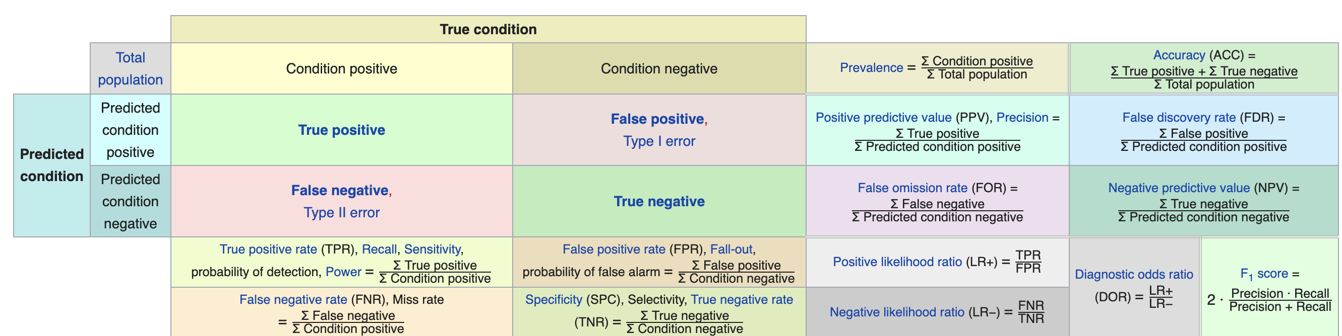
图8.1: 混淆矩阵
这里我要着重介绍一下这个表的意义,这个表格的上方的Ture condition的意思就等同于这里的真实值, 而右边的Predicted condition就等同于这里的预测值的意思,True positive 和True negative就代表的真阳性和真阴性的值,而False positive 和 False negative则表示假阳性和假阴性的意思,判定这个预测模型的优良,有五个指标至关重要,主要包括sensitivity, speciticity,precision,negative predictive value以及accuracy。其中,sensitivity是指预测一个因子的敏感度,表达的是认为是正类并且确实是正类的部分占所有确实是正类的比例,也有的表达为recall, 是相对真实的情况而言的。 speciticity是指模型能指定地判断出阴性的能力,也叫真阴性率。precision是精确度的意思,精确度表示我们预测的阳性结果中是真阳性的比例。 negative predictive value是指真阴性的预测比例,与精确度正好相反,是表示我们预测的阴性结果中是真阴性的比例。下图是详细的介绍:
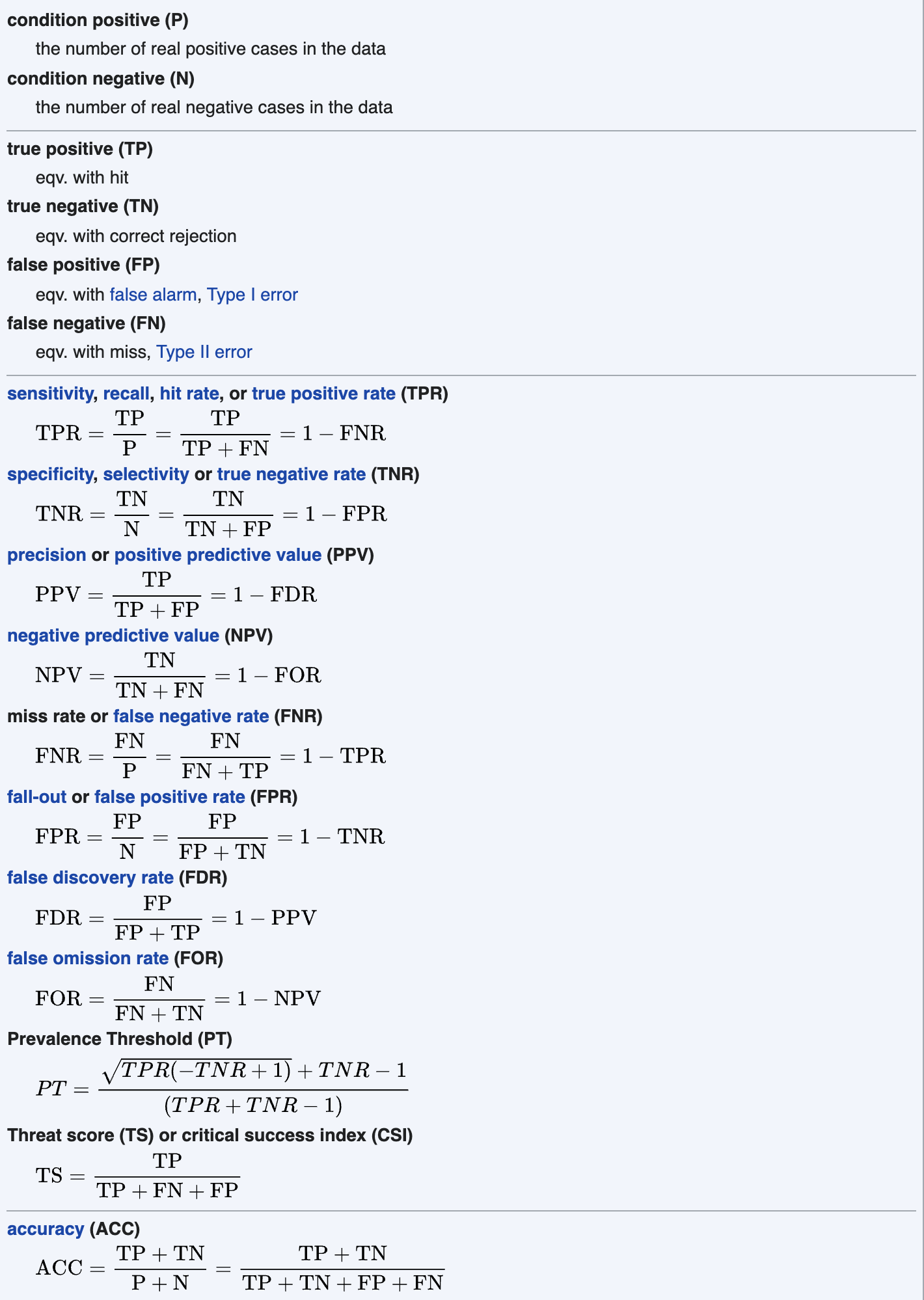
图8.2: 判定模型相关指标
有了对这方面的认知,我们回过头来看我们用模型预测val数据得到的结果第二项,Overall Statistics,这一项包括了我们这个模型的总的准确率等一些最终结果,接下来第三项是 Statistics by Class,这一项包括了所有以上提到的4个重要判定指标,主要包括:sensitivity, speciticity,precision,negative predictive value。 对于一个判定模型,其对验证集的预测能力判定主要依靠以上几个指标进行综合判定。到这里我们就可以得到了用原始数据的建模及模型判定能力指标的结果。接下来我们看一下用其他预处理过的光谱数据建模是否可以有效提高判别模型的判定能力。这里我们使用一阶导数处理后的数据。
library(e1071)
library(prospectr)
#提取光谱数据和其已知种源信息
nir <- as.matrix(spec[,-c(1:2,238:258)])
fst_der <- savitzkyGolay(nir,1,2,15)
orig <- spec$typee
#用这两个指标构建一个新的dataframe 数据

data_new <- data.frame(y=orig,x=fst_der)

### split 数据为训练集和验证集,以便检测模型稳定性
library(caret)
int <- createDataPartition(data_new$y, p = .80,list=F)
train <- data_new[int,]
val  <- data_new[-int,]
#构建svm判别模型
library(e1071)
svm_1st = svm(y ~ ., data = train,
               kernel = "radial", cost = 64,epsilon=0, scale = T)
#y~.的意思是y是四种种源的信息,
#波浪号后面跟个英文句点是代表后面使用全部的数据。
#这里我们用radial方法进行模型构建。
#你也可以选择其他的判别方法,可以通过 ?svm 进入help页进行详细查询。
#得到的模型我们可以通过summary来看看模型的性质。
summary(svm_1st)
##
## Call:
## svm(formula = y ~ ., data = train, kernel = "radial", cost = 64,
## epsilon = 0, scale = T)
##
##
## Parameters:
## SVM-Type: C-classification
## SVM-Kernel: radial
## cost: 64
##
## Number of Support Vectors: 365
##
## ( 115 57 137 56 )
##
##
## Number of Classes: 4
##
## Levels:
## BJ G P S得到模型后,使用val数据对模型进行检验。
pred_test <- predict(svm_1st,val)
##接下来我们用真实值和预测值构建confusion matrix,来看看模型的预测能力怎么样
confusionMatrix(data = pred_test, val$y)
## Confusion Matrix and Statistics
##
## Reference
## Prediction BJ G P S
## BJ 51 0 5 1
## G 0 22 1 0
## P 1 1 42 0
## S 2 0 0 23
##
## Overall Statistics
##
## Accuracy : 0.9262
## 95% CI : (0.8717, 0.9626)
## No Information Rate : 0.3624
## P-Value [Acc > NIR] : < 2.2e-16
##
## Kappa : 0.8968
##
## Mcnemar's Test P-Value : NA
##
## Statistics by Class:
##
## Class: BJ Class: G Class: P Class: S
## Sensitivity 0.9444 0.9565 0.8750 0.9583
## Specificity 0.9368 0.9921 0.9802 0.9840
## Pos Pred Value 0.8947 0.9565 0.9545 0.9200
## Neg Pred Value 0.9674 0.9921 0.9429 0.9919
## Prevalence 0.3624 0.1544 0.3221 0.1611
## Detection Rate 0.3423 0.1477 0.2819 0.1544
## Detection Prevalence 0.3826 0.1544 0.2953 0.1678
## Balanced Accuracy 0.9406 0.9743 0.9276 0.9712### confusionmatrix 来自library(caret)
从结果来看,经过一阶导数处理后的光谱数据建立的判别模型,其准确率要大于原始光谱构建的模型,说明不同的预处理对模型的精度产生了影响,同时,你会发现,每次分出来的train和val数据是不一样的,所得的预测结果的准确率也是不一样的,那是因为这个数据筛选的过程是随机的,它是根据你所想要选择的强度,进行筛选,不保证每次筛选出来的是一样的,如果想让每次筛选的一样,你可以用以下这个代码,设置固定的seed。比如:
library(caret)
set.seed(1234)## 为了确保随机选择的结果是一致的
int <- createDataPartition(data_new$y, p = .80,list=F)
head(int)
## Resample1
## [1,] 1
## [2,] 2
## [3,] 3
## [4,] 4
## [5,] 6
## [6,] 7library(prospectr)
这样你每次筛选的就会是同样的数据,这里是方便让结果一致,以免造成后续数据无法相同,引起不必要的麻烦,当然,除了随机筛选数据的方法,我们还可以使用其他固定筛选train和 val数据的方法,比如Kennard-Stone algorithm算法, 这种算法可以选择出均匀分布的样品,确保选择样品最大化代表整体样品。 这个方法我们可以通过prospectr这个安装包里面的kenStone程序实现,具体如下:
library(prospectr)
sel <- kenStone(data_new[-1], k = 598,'mahal' , pc = .99)
plot(sel$pc[, 1:2], xlab = 'PC1', ylab = 'PC2')
points(sel$pc[sel$model, 1:2], pch = 19, col = 2) # points selected for calibration 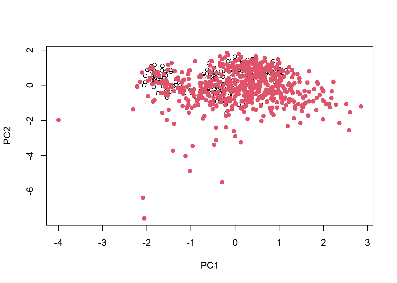
train <- data_new [sel$model,]
test <- data_new[sel$test,]
这样选择出来的训练集最大程度的代表了整体的数据,因此可以进行下一步的模型构建和验证,到这个时候我们基本上已经完成了模型构建和验证,如果验证的模型准确度很高,就可以用光谱数据来反演预测其他未知数据。
8.1.2 RF模型
首先,让我们来看看维基百科是怎么解释随机森林模型的: >在机器学习中,随机森林是一个包含多个决策树的分类器,并且其输出的类别是由个别树输出的类别的众数而定。 这个术语是1995年[1]由贝尔实验室的何天琴所提出的随机决策森林(random decision forests)而来的 然后Leo Breiman和Adele Cutler发展出推论出随机森林的算法。而“Random Forests”是他们的商标。 这个方法则是结合Breimans的“Bootstrap aggregating”想法和Ho的“random subspace method”以建造决策树的集合。
我这里也把链接放在这里,有兴趣了解详情的,可以点击以下连接:随机森林模型,我这里就不做过多的介绍,它的最大优点是:1,它速度快且可以处理大量的输入变量;2,它可以再决定类别的时候,评估变量的重要性,这个对于我们找到重要变量很重要;3,它可以很好的处理不平衡数据。这个方法也被广泛地应用于判别分析当中,我这里着重讲一下如何再R里面实现。
R里面有很多比较成熟的安装包可以实现RF,这里我主要介绍一下ranger这个安装包,这个安装包里的ranger这个程序可以用来做RF模型,接下来我们来继续拿 8.1.1原始光谱数据进行举例,首先还是讲数据分为训练集和验证集:
#提取光谱数据和其已知种源信息
nir <- as.matrix(spec[,-c(1:2,238:258)])
orig <- spec$typee
#用这两个指标构建一个新的dataframe 数据

data_new <- data.frame(y=orig,x=fst_der)

### split 数据为训练集和验证集,以便检测模型稳定性
library(caret)
int <- createDataPartition(data_new$y, p = .80,list=F)
train <- data_new[int,]
val  <- data_new[-int,]

library(ranger)
rf_fit =  ranger(y ~ ., data = train,  importance = "impurity",
                   scale = T)
print(rf_fit)
## Ranger result
##
## Call:
## ranger(y ~ ., data = train, importance = "impurity", scale = T)
##
## Type: Classification
## Number of trees: 500
## Sample size: 598
## Number of independent variables: 221
## Mtry: 14
## Target node size: 1
## Variable importance mode: impurity
## Splitrule: gini
## OOB prediction error: 14.38 %###预测验证集
pred_val <- predict(rf_fit,val)
pred_val$predictions#查看数据## [1] BJ BJ BJ BJ BJ BJ BJ BJ BJ BJ BJ BJ BJ BJ BJ BJ BJ BJ BJ BJ BJ BJ BJ BJ BJ
## [26] BJ BJ BJ BJ BJ BJ BJ BJ BJ BJ BJ BJ BJ BJ BJ BJ BJ BJ BJ BJ BJ BJ BJ BJ P
## [51] P P P S P G G G G G G G G P G G G G G G G G G G G
## [76] G G BJ P P P P P P P P S BJ P BJ P P P P P P P P P P
## [101] S S BJ S S S BJ S P S S BJ S S S BJ BJ S S S S S S S P
## [126] P P P P P P P S G P P P P P P P P P P P BJ P P P
## Levels: BJ G P S#混淆矩阵
confmat <-confusionMatrix(data = pred_val$predictions, as.factor(val[,1]))
confmat ## Confusion Matrix and Statistics
##
## Reference
## Prediction BJ G P S
## BJ 49 0 4 5
## G 0 21 1 0
## P 4 2 41 1
## S 1 0 2 18
##
## Overall Statistics
##
## Accuracy : 0.8658
## 95% CI : (0.8003, 0.916)
## No Information Rate : 0.3624
## P-Value [Acc > NIR] : < 2.2e-16
##
## Kappa : 0.8109
##
## Mcnemar's Test P-Value : NA
##
## Statistics by Class:
##
## Class: BJ Class: G Class: P Class: S
## Sensitivity 0.9074 0.9130 0.8542 0.7500
## Specificity 0.9053 0.9921 0.9307 0.9760
## Pos Pred Value 0.8448 0.9545 0.8542 0.8571
## Neg Pred Value 0.9451 0.9843 0.9307 0.9531
## Prevalence 0.3624 0.1544 0.3221 0.1611
## Detection Rate 0.3289 0.1409 0.2752 0.1208
## Detection Prevalence 0.3893 0.1477 0.3221 0.1409
## Balanced Accuracy 0.9063 0.9526 0.8924 0.8630
可以看出,我们原始数据的RF判别模型的准确度还是不错的,我们把判别模型的主要指标提取出来,就可以进行比较模型得准确性,接下来我们来看看重要的变量:
var_impor <- ranger::importance (rf_fit)
var_impor
## x.1015.5 x.1021.3 x.1027.2 x.1033.1 x.1039 x.1045 x.1051.1
## 7.6195371 6.4494393 4.2324185 5.0328703 5.3300395 6.6937008 7.7794738
## x.1057.2 x.1063.2 x.1069.4 x.1075.5 x.1081.7 x.1087.9 x.1094.2
## 7.5579210 5.1703855 3.8307153 2.8893742 1.5172280 1.2105025 0.9481631
## x.1100.4 x.1106.7 x.1113 x.1119.3 x.1125.6 x.1131.9 x.1138.2
## 0.8920622 0.6527534 0.7467495 0.8329238 0.6943016 0.9432146 0.9286609
## x.1144.6 x.1151 x.1157.3 x.1163.7 x.1170 x.1176.4 x.1182.8
## 1.1502521 0.9990028 1.4236132 1.5369446 1.7551294 2.0150290 1.7226367
## x.1189.1 x.1195.5 x.1201.9 x.1208.2 x.1214.6 x.1221 x.1227.3
## 2.0212198 2.0385031 2.1085500 2.0624718 3.4438620 2.7009493 2.0944525
## x.1233.7 x.1240 x.1246.4 x.1252.7 x.1259 x.1265.3 x.1271.6
## 1.8086251 2.8851788 2.6027260 2.8930850 1.9969980 2.1656116 1.4784374
## x.1277.9 x.1284.2 x.1290.5 x.1296.8 x.1303 x.1309.3 x.1315.5
## 1.5428845 0.8966864 0.8768882 0.6665023 1.0175625 0.7353802 0.7662507
## x.1321.8 x.1328 x.1334.2 x.1340.4 x.1346.6 x.1352.8 x.1359
## 0.7415311 0.7391068 0.9101385 1.1917357 1.3080654 1.2384615 1.2850041
## x.1365.1 x.1371.3 x.1377.4 x.1383.5 x.1389.7 x.1395.8 x.1401.9
## 0.9528717 0.8488600 0.7548313 0.8888601 0.7015868 0.6062677 0.6908855
## x.1408 x.1414 x.1420.1 x.1426.2 x.1432.2 x.1438.3 x.1444.3
## 0.6631239 0.5013040 0.7176044 0.6678701 0.6702601 0.6971941 0.7740321
## x.1450.4 x.1456.4 x.1462.4 x.1468.4 x.1474.4 x.1480.4 x.1486.4
## 1.3198231 1.4254750 2.3665247 2.9648519 2.0753344 1.6935474 0.8567548
## x.1492.4 x.1498.4 x.1504.3 x.1510.3 x.1516.2 x.1522.2 x.1528.2
## 0.7655772 0.6218462 0.4636017 0.6253790 0.3972331 0.4102398 0.5144806
## x.1534.1 x.1540.1 x.1546 x.1551.9 x.1557.9 x.1563.8 x.1569.8
## 0.5849809 0.6090926 0.6407893 0.7529878 0.7205698 0.9646842 1.0059238
## x.1575.7 x.1581.6 x.1587.5 x.1593.5 x.1599.4 x.1605.3 x.1611.2
## 1.0185866 1.2498484 1.2679464 1.2312360 1.2501921 1.2206961 1.4494426
## x.1617.2 x.1623.1 x.1629 x.1635 x.1640.9 x.1646.8 x.1652.8
## 1.5246869 1.4725290 1.3638736 1.5797369 1.3793817 1.8192929 2.8327601
## x.1658.7 x.1664.6 x.1670.6 x.1676.5 x.1682.5 x.1688.4 x.1694.4
## 3.4351848 3.6962782 5.2323870 5.9696303 6.5810040 5.8763246 5.8271805
## x.1700.3 x.1706.3 x.1712.2 x.1718.2 x.1724.2 x.1730.2 x.1736.1
## 7.1619149 7.1433599 4.5017335 5.4351780 7.0770141 8.4430062 8.1250490
## x.1742.1 x.1748.1 x.1754.1 x.1760.1 x.1766.1 x.1772.1 x.1778.1
## 10.1225461 7.0086982 6.4456605 5.7699019 5.3645486 4.2315270 4.0032262
## x.1784.1 x.1790.1 x.1796.1 x.1802.1 x.1808.2 x.1814.2 x.1820.2
## 2.7059800 2.4699649 1.3049867 1.3238793 1.7365898 2.5014196 2.9925453
## x.1826.3 x.1832.3 x.1838.4 x.1844.4 x.1850.5 x.1856.5 x.1862.6
## 2.7399071 2.5916870 2.6277331 2.2304629 1.6719748 1.3925598 0.9047535
## x.1868.6 x.1874.7 x.1880.8 x.1886.8 x.1892.9 x.1899 x.1905.1
## 0.8496040 0.9758449 0.9615856 1.4049426 1.4095788 1.5224494 1.5129336
## x.1911.2 x.1917.2 x.1923.3 x.1929.4 x.1935.5 x.1941.6 x.1947.7
## 2.0505418 2.0807644 2.1423968 1.7965645 1.1068040 0.9132524 0.8089306
## x.1953.8 x.1959.8 x.1965.9 x.1972 x.1978.1 x.1984.2 x.1990.3
## 0.9219090 0.6303393 0.6516294 0.5973626 0.7132372 0.6772315 0.6149686
## x.1996.4 x.2002.5 x.2008.5 x.2014.6 x.2020.7 x.2026.8 x.2032.9
## 0.6325050 0.6774666 0.8503750 1.3670420 1.3873907 1.2611830 1.2932039
## x.2038.9 x.2045 x.2051.1 x.2057.1 x.2063.2 x.2069.2 x.2075.3
## 1.3245791 1.7769285 1.5163974 1.4926103 1.2156622 1.0171997 0.9172358
## x.2081.3 x.2087.4 x.2093.4 x.2099.4 x.2105.5 x.2111.5 x.2117.5
## 0.7443287 0.6276063 0.5940434 0.6908828 0.6465596 0.7309260 0.7874204
## x.2123.5 x.2129.5 x.2135.5 x.2141.5 x.2147.5 x.2153.5 x.2159.5
## 0.9277146 0.9687372 0.8336601 0.9107742 1.0671300 0.9973177 1.0098706
## x.2165.4 x.2171.4 x.2177.4 x.2183.3 x.2189.3 x.2195.2 x.2201.2
## 0.9932314 1.1742590 1.2012371 1.1424527 0.9947704 0.9718714 1.5634626
## x.2207.1 x.2213.1 x.2219 x.2224.9 x.2230.8 x.2236.8 x.2242.7
## 1.3104600 1.6126116 1.3543570 1.6669206 2.0040529 1.9486562 1.5176720
## x.2248.6 x.2254.5 x.2260.4 x.2266.3 x.2272.3 x.2278.2 x.2284.1
## 1.4591566 1.4007073 1.2854311 1.0158036 0.9513698 0.9768899 0.8737902
## x.2290 x.2295.9 x.2301.8 x.2307.8 x.2313.7 x.2319.6 x.2325.6
## 0.6538682 0.5349014 0.7010234 0.6984176 0.7077653 0.7904271 0.6066288
## x.2331.5 x.2337.5 x.2343.5 x.2349.5
## 0.9335126 1.1457375 1.0663954 1.0432646as.numeric(gsub('x.','' ,names(var_impor)))## [1] 1015.5 1021.3 1027.2 1033.1 1039.0 1045.0 1051.1 1057.2 1063.2 1069.4
## [11] 1075.5 1081.7 1087.9 1094.2 1100.4 1106.7 1113.0 1119.3 1125.6 1131.9
## [21] 1138.2 1144.6 1151.0 1157.3 1163.7 1170.0 1176.4 1182.8 1189.1 1195.5
## [31] 1201.9 1208.2 1214.6 1221.0 1227.3 1233.7 1240.0 1246.4 1252.7 1259.0
## [41] 1265.3 1271.6 1277.9 1284.2 1290.5 1296.8 1303.0 1309.3 1315.5 1321.8
## [51] 1328.0 1334.2 1340.4 1346.6 1352.8 1359.0 1365.1 1371.3 1377.4 1383.5
## [61] 1389.7 1395.8 1401.9 1408.0 1414.0 1420.1 1426.2 1432.2 1438.3 1444.3
## [71] 1450.4 1456.4 1462.4 1468.4 1474.4 1480.4 1486.4 1492.4 1498.4 1504.3
## [81] 1510.3 1516.2 1522.2 1528.2 1534.1 1540.1 1546.0 1551.9 1557.9 1563.8
## [91] 1569.8 1575.7 1581.6 1587.5 1593.5 1599.4 1605.3 1611.2 1617.2 1623.1
## [101] 1629.0 1635.0 1640.9 1646.8 1652.8 1658.7 1664.6 1670.6 1676.5 1682.5
## [111] 1688.4 1694.4 1700.3 1706.3 1712.2 1718.2 1724.2 1730.2 1736.1 1742.1
## [121] 1748.1 1754.1 1760.1 1766.1 1772.1 1778.1 1784.1 1790.1 1796.1 1802.1
## [131] 1808.2 1814.2 1820.2 1826.3 1832.3 1838.4 1844.4 1850.5 1856.5 1862.6
## [141] 1868.6 1874.7 1880.8 1886.8 1892.9 1899.0 1905.1 1911.2 1917.2 1923.3
## [151] 1929.4 1935.5 1941.6 1947.7 1953.8 1959.8 1965.9 1972.0 1978.1 1984.2
## [161] 1990.3 1996.4 2002.5 2008.5 2014.6 2020.7 2026.8 2032.9 2038.9 2045.0
## [171] 2051.1 2057.1 2063.2 2069.2 2075.3 2081.3 2087.4 2093.4 2099.4 2105.5
## [181] 2111.5 2117.5 2123.5 2129.5 2135.5 2141.5 2147.5 2153.5 2159.5 2165.4
## [191] 2171.4 2177.4 2183.3 2189.3 2195.2 2201.2 2207.1 2213.1 2219.0 2224.9
## [201] 2230.8 2236.8 2242.7 2248.6 2254.5 2260.4 2266.3 2272.3 2278.2 2284.1
## [211] 2290.0 2295.9 2301.8 2307.8 2313.7 2319.6 2325.6 2331.5 2337.5 2343.5
## [221] 2349.5###我们可以把它绘图出来
matplot( as.numeric(gsub('x.','' ,names(var_impor))),
pch=16,
var_impor,type = 'b')#type=b,是Both的意思,就是既有点,又有线。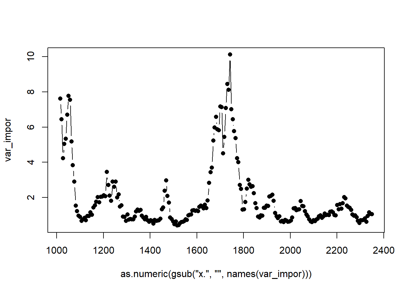
通过查看最优变量,我们可以找到对模型判别准确率贡献最大的光谱波段,然后进行进一步筛选,保留最优变量,然后重新建模,这样的好处,可以减少无用信息的输入,大大减少运算时间,也可以为以后特定光谱相机构建作为指导。到这里,就是RF模型的构建及验证,作图了,如果想了解具体这个ranger程序都有什么参数可以调节,可以用?ranger来调出来帮助页码,可以很好的理解。接下来就是另一个判别模型的介绍了。
8.1.3 DT模型
决策树也是一个比较常用并且简单的模型方法,其可以用来作为判别模型,也可以用来作为回归模型,其作为判别模型的时候,有以下几个优点,这里简单介绍一下:
1, 非常容易理解; 2, 可以很好的处理缺失和异常值,减少了前期数据清洗的时间; 3,可以很好的处理分类,减少了人工分类的时间; 4,决策树还可以对非线性关系进行建模,非常实用。
但是事物一般分两面性,它可以很简单,也可以很复杂,复杂的决策树可能会导致模型过拟合,导致模型准确性降低。但是不管怎么说,大部分情况下,它还是一个比较好的判别模型方法,接下来我们就用我们的数据进行一下决策树建模。这里我们要用到rpart和rpart.plot这两个安装包进行决策树模型构建。当然安装包caret非常强大,可以做很多模型运算,感兴趣的读者可以去了解一下这本电子书The caret Package,里面有非常详细的介绍,这里因为想让大家具体简单了解一下,因此就没有用到caret这个包里面的模型运算。
#提取光谱数据和其已知种源信息
nir <- as.matrix(spec[,-c(1:2,238:258)])
orig <- spec$typee
#用这两个指标构建一个新的dataframe 数据

data_new <- data.frame(y=orig,x=fst_der)

### split 数据为训练集和验证集,以便检测模型稳定性
library(caret)
int <- createDataPartition(data_new$y, p = .80,list=F)
train <- data_new[int,]
val  <- data_new[-int,]

library(rpart)
library(rpart.plot)
dt_fit =  rpart(y ~ ., data = train,  method = 'class')
rpart.plot(dt_fit)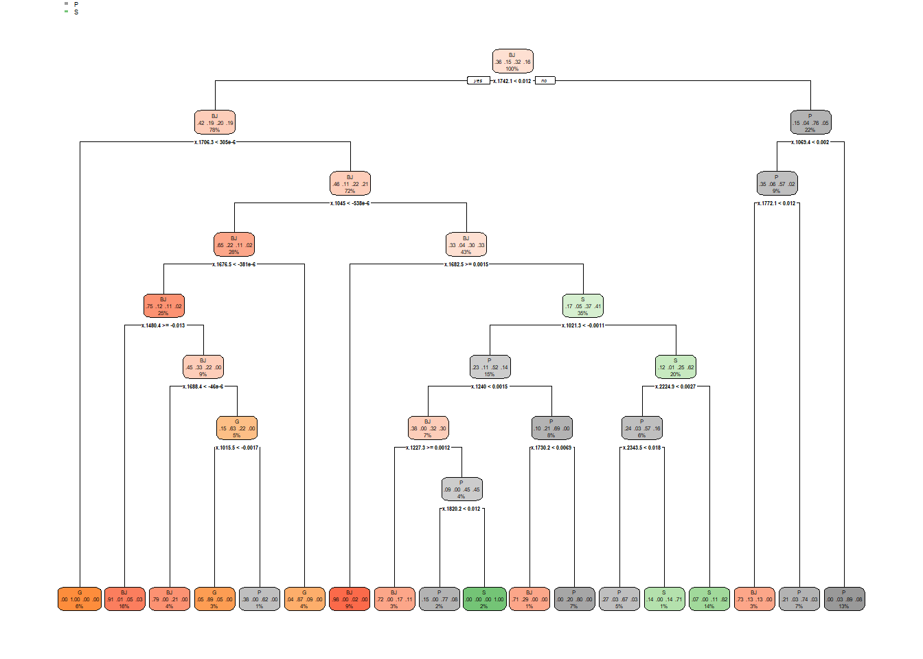
###预测验证集

pred_val <- predict(dt_fit,val, type = 'class')
#混淆矩阵
confmat <-confusionMatrix(data =  pred_val, as.factor(val[,1]))
confmat
## Confusion Matrix and Statistics
##
## Reference
## Prediction BJ G P S
## BJ 41 3 7 1
## G 0 19 2 0
## P 9 1 36 7
## S 4 0 3 16
##
## Overall Statistics
##
## Accuracy : 0.7517
## 95% CI : (0.6743, 0.8187)
## No Information Rate : 0.3624
## P-Value [Acc > NIR] : < 2.2e-16
##
## Kappa : 0.6514
##
## Mcnemar's Test P-Value : NA
##
## Statistics by Class:
##
## Class: BJ Class: G Class: P Class: S
## Sensitivity 0.7593 0.8261 0.7500 0.6667
## Specificity 0.8842 0.9841 0.8317 0.9440
## Pos Pred Value 0.7885 0.9048 0.6792 0.6957
## Neg Pred Value 0.8660 0.9688 0.8750 0.9365
## Prevalence 0.3624 0.1544 0.3221 0.1611
## Detection Rate 0.2752 0.1275 0.2416 0.1074
## Detection Prevalence 0.3490 0.1409 0.3557 0.1544
## Balanced Accuracy 0.8217 0.9051 0.7908 0.8053看来DT模型的结果不是太好,模型准确度相对于其他两个模型来说,不是太高,当然,这不代表这个方法就不好,不同的数据及运算要求,可能会对算法有不同的要求,因此,找到适合自己数据的模型最重要。这图大致讲的意思就是类似于做选择题,它会根据各种条件,进行判断,比如是和否,然后根据是和否的条件再做选择,最终进行判别。 这里就简单介绍到这里。如果有其他疑问,我们后续可以再讨论。
8.1.4 ANN 模型
神经网络是一种模拟人类思维的计算设计。与ANN相比,支持向量机首先将输入数据概述到由核函数定义的高维特征空间中,然后找到可以最大程度地分布训练数据的最好超平面。该过程是通过使用人工神经网络(ANN)进行的。人工神经网络被认为是计算世界中最有用的技术之一。 虽然有人说这是一个黑匣子,无法了解里面的具体过程,但很多研究已经在R语言里面开发ANN。
在R语言当中,实现ANN 判别模型,我们需要用到nnet这个安装包,其代码过程跟前面几个模型类似。
#提取光谱数据和其已知种源信息
nir <- as.matrix(spec[,-c(1:2,238:258)])
orig <- spec$typee
#用这两个指标构建一个新的dataframe 数据

data_new <- data.frame(y=orig,x=fst_der)

### split 数据为训练集和验证集,以便检测模型稳定性
library(caret)
int <- createDataPartition(data_new$y, p = .80,list=F)
train <- data_new[int,]
val  <- data_new[-int,]

library(nnet)
n <- names(train)
f <- as.formula(paste("y ~", paste(n[!n %in% "y"], collapse = " + ")))
ann_fit =  nnet(f, data = train, size = 4,decay = 0.0001,maxit = 500)
## # weights: 908
## initial value 795.934607
## iter 10 value 773.179735
## iter 20 value 714.892518
## iter 30 value 625.758609
## iter 40 value 481.192693
## iter 50 value 376.549758
## iter 60 value 245.681919
## iter 70 value 149.038500
## iter 80 value 103.291911
## iter 90 value 75.346788
## iter 100 value 61.879789
## iter 110 value 49.954892
## iter 120 value 43.432001
## iter 130 value 39.640631
## iter 140 value 36.206418
## iter 150 value 34.111076
## iter 160 value 32.213468
## iter 170 value 31.102231
## iter 180 value 30.004937
## iter 190 value 29.288146
## iter 200 value 28.864275
## iter 210 value 28.565388
## iter 220 value 28.283522
## iter 230 value 28.113582
## iter 240 value 27.976721
## iter 250 value 27.876638
## iter 260 value 27.815280
## iter 270 value 27.726107
## iter 280 value 27.663301
## iter 290 value 27.596068
## iter 300 value 27.514545
## iter 310 value 27.452839
## iter 320 value 27.385982
## iter 330 value 27.330966
## iter 340 value 27.243441
## iter 350 value 27.047701
## iter 360 value 26.905207
## iter 370 value 26.763860
## iter 380 value 26.606086
## iter 390 value 26.393262
## iter 400 value 26.246955
## iter 410 value 26.172184
## iter 420 value 26.039734
## iter 430 value 25.907813
## iter 440 value 25.814818
## iter 450 value 25.740882
## iter 460 value 25.642108
## iter 470 value 25.571716
## iter 480 value 25.485960
## iter 490 value 25.390948
## iter 500 value 25.311147
## final value 25.311147
## stopped after 500 iterationssummary(ann_fit)## a 221-4-4 network with 908 weights
## options were - softmax modelling decay=1e-04
## b->h1 i1->h1 i2->h1 i3->h1 i4->h1 i5->h1 i6->h1 i7->h1
## 15.34 12.42 9.79 4.04 1.55 1.83 -2.68 -4.58
## i8->h1 i9->h1 i10->h1 i11->h1 i12->h1 i13->h1 i14->h1 i15->h1
## -6.24 -8.76 -7.78 -6.02 -5.12 -4.89 -4.17 -5.41
## i16->h1 i17->h1 i18->h1 i19->h1 i20->h1 i21->h1 i22->h1 i23->h1
## -5.31 -3.18 -3.59 -3.76 -1.88 -1.16 -0.61 -1.16
## i24->h1 i25->h1 i26->h1 i27->h1 i28->h1 i29->h1 i30->h1 i31->h1
## -1.82 -1.35 -0.90 -1.08 -1.95 -2.51 -4.55 -5.71
## i32->h1 i33->h1 i34->h1 i35->h1 i36->h1 i37->h1 i38->h1 i39->h1
## -5.71 -5.66 -5.35 -4.68 -3.73 -2.78 -2.40 -2.14
## i40->h1 i41->h1 i42->h1 i43->h1 i44->h1 i45->h1 i46->h1 i47->h1
## -2.40 -2.61 -2.38 -1.87 -1.14 -0.72 -1.51 -3.05
## i48->h1 i49->h1 i50->h1 i51->h1 i52->h1 i53->h1 i54->h1 i55->h1
## -1.87 -1.95 -3.31 -4.88 -6.95 -9.13 -11.15 -12.87
## i56->h1 i57->h1 i58->h1 i59->h1 i60->h1 i61->h1 i62->h1 i63->h1
## -15.86 -17.96 -17.87 -17.12 -16.78 -15.73 -15.54 -13.90
## i64->h1 i65->h1 i66->h1 i67->h1 i68->h1 i69->h1 i70->h1 i71->h1
## -12.83 -11.53 -6.91 -4.47 -2.76 -2.15 0.25 0.97
## i72->h1 i73->h1 i74->h1 i75->h1 i76->h1 i77->h1 i78->h1 i79->h1
## 0.70 3.85 4.65 2.42 4.44 5.61 3.16 0.43
## i80->h1 i81->h1 i82->h1 i83->h1 i84->h1 i85->h1 i86->h1 i87->h1
## -1.38 -0.01 -0.67 -2.87 -5.36 -4.48 -4.14 -4.28
## i88->h1 i89->h1 i90->h1 i91->h1 i92->h1 i93->h1 i94->h1 i95->h1
## -1.76 -0.97 -2.55 0.40 2.91 2.05 2.99 3.93
## i96->h1 i97->h1 i98->h1 i99->h1 i100->h1 i101->h1 i102->h1 i103->h1
## 4.45 3.44 2.53 -0.85 -3.97 -4.16 -6.05 -7.77
## i104->h1 i105->h1 i106->h1 i107->h1 i108->h1 i109->h1 i110->h1 i111->h1
## -7.25 -6.84 -4.78 -1.81 -1.36 0.66 1.89 1.51
## i112->h1 i113->h1 i114->h1 i115->h1 i116->h1 i117->h1 i118->h1 i119->h1
## 3.91 4.48 2.11 1.39 1.69 2.12 1.02 1.02
## i120->h1 i121->h1 i122->h1 i123->h1 i124->h1 i125->h1 i126->h1 i127->h1
## 3.16 3.51 4.11 3.89 4.99 4.24 2.58 2.02
## i128->h1 i129->h1 i130->h1 i131->h1 i132->h1 i133->h1 i134->h1 i135->h1
## -1.41 -0.74 -3.58 -7.63 -4.83 -7.31 -3.15 8.12
## i136->h1 i137->h1 i138->h1 i139->h1 i140->h1 i141->h1 i142->h1 i143->h1
## 10.68 11.57 12.45 16.33 9.93 -4.61 -6.21 -6.92
## i144->h1 i145->h1 i146->h1 i147->h1 i148->h1 i149->h1 i150->h1 i151->h1
## -2.89 5.55 -8.94 -5.46 -9.41 -4.39 0.05 -10.52
## i152->h1 i153->h1 i154->h1 i155->h1 i156->h1 i157->h1 i158->h1 i159->h1
## 10.91 6.88 6.22 8.61 -6.95 -5.66 -3.75 2.30
## i160->h1 i161->h1 i162->h1 i163->h1 i164->h1 i165->h1 i166->h1 i167->h1
## 19.36 10.31 15.89 21.64 25.44 19.83 18.95 30.40
## i168->h1 i169->h1 i170->h1 i171->h1 i172->h1 i173->h1 i174->h1 i175->h1
## 3.31 5.80 9.99 7.09 16.84 14.07 17.09 14.87
## i176->h1 i177->h1 i178->h1 i179->h1 i180->h1 i181->h1 i182->h1 i183->h1
## 12.25 12.71 14.00 18.10 1.04 11.07 13.43 -16.87
## i184->h1 i185->h1 i186->h1 i187->h1 i188->h1 i189->h1 i190->h1 i191->h1
## -12.45 -5.22 -12.94 -13.31 -9.12 -9.28 -15.89 -8.71
## i192->h1 i193->h1 i194->h1 i195->h1 i196->h1 i197->h1 i198->h1 i199->h1
## -7.67 -1.75 6.94 -10.95 -12.59 3.32 1.10 -0.93
## i200->h1 i201->h1 i202->h1 i203->h1 i204->h1 i205->h1 i206->h1 i207->h1
## 10.79 15.19 8.81 12.65 6.64 -1.57 18.94 -0.14
## i208->h1 i209->h1 i210->h1 i211->h1 i212->h1 i213->h1 i214->h1 i215->h1
## -1.08 7.38 13.71 9.50 -10.74 0.41 2.60 1.09
## i216->h1 i217->h1 i218->h1 i219->h1 i220->h1 i221->h1
## 12.82 -21.95 -17.40 7.35 -9.37 -4.67
## b->h2 i1->h2 i2->h2 i3->h2 i4->h2 i5->h2 i6->h2 i7->h2
## 2.28 -20.43 -14.46 -4.98 -1.57 -0.79 9.26 13.21
## i8->h2 i9->h2 i10->h2 i11->h2 i12->h2 i13->h2 i14->h2 i15->h2
## 15.97 19.82 17.52 12.40 9.39 5.60 0.25 0.28
## i16->h2 i17->h2 i18->h2 i19->h2 i20->h2 i21->h2 i22->h2 i23->h2
## -1.29 -7.72 -11.73 -16.25 -22.95 -25.80 -25.75 -25.47
## i24->h2 i25->h2 i26->h2 i27->h2 i28->h2 i29->h2 i30->h2 i31->h2
## -24.84 -23.97 -22.33 -19.07 -15.25 -12.03 -5.68 -0.80
## i32->h2 i33->h2 i34->h2 i35->h2 i36->h2 i37->h2 i38->h2 i39->h2
## 1.63 3.22 3.66 2.49 -0.04 -1.24 -2.34 -3.00
## i40->h2 i41->h2 i42->h2 i43->h2 i44->h2 i45->h2 i46->h2 i47->h2
## -3.24 -3.44 -4.94 -8.24 -11.02 -12.46 -13.50 -12.29
## i48->h2 i49->h2 i50->h2 i51->h2 i52->h2 i53->h2 i54->h2 i55->h2
## -13.32 -13.32 -10.59 -7.68 -3.71 0.27 3.67 7.20
## i56->h2 i57->h2 i58->h2 i59->h2 i60->h2 i61->h2 i62->h2 i63->h2
## 10.90 13.59 10.18 3.55 2.36 0.15 -0.47 0.52
## i64->h2 i65->h2 i66->h2 i67->h2 i68->h2 i69->h2 i70->h2 i71->h2
## 3.85 6.31 0.93 -0.34 2.92 6.12 5.98 6.95
## i72->h2 i73->h2 i74->h2 i75->h2 i76->h2 i77->h2 i78->h2 i79->h2
## 8.25 4.74 1.01 4.72 1.73 -2.53 1.50 7.21
## i80->h2 i81->h2 i82->h2 i83->h2 i84->h2 i85->h2 i86->h2 i87->h2
## 10.15 4.14 3.22 9.53 14.30 12.94 12.22 10.62
## i88->h2 i89->h2 i90->h2 i91->h2 i92->h2 i93->h2 i94->h2 i95->h2
## 8.30 6.67 9.21 6.54 0.63 1.14 -2.98 -7.68
## i96->h2 i97->h2 i98->h2 i99->h2 i100->h2 i101->h2 i102->h2 i103->h2
## -10.51 -9.15 -5.79 -3.09 0.31 3.37 4.76 8.34
## i104->h2 i105->h2 i106->h2 i107->h2 i108->h2 i109->h2 i110->h2 i111->h2
## 8.01 4.76 1.50 -4.81 -5.03 -9.23 -11.42 -7.99
## i112->h2 i113->h2 i114->h2 i115->h2 i116->h2 i117->h2 i118->h2 i119->h2
## -8.86 -5.17 1.48 6.08 10.37 9.30 13.05 17.21
## i120->h2 i121->h2 i122->h2 i123->h2 i124->h2 i125->h2 i126->h2 i127->h2
## 15.83 14.24 12.73 13.19 8.93 8.88 11.17 0.08
## i128->h2 i129->h2 i130->h2 i131->h2 i132->h2 i133->h2 i134->h2 i135->h2
## -5.19 -1.61 -0.36 2.19 2.25 15.97 18.43 2.66
## i136->h2 i137->h2 i138->h2 i139->h2 i140->h2 i141->h2 i142->h2 i143->h2
## 2.65 5.78 -4.21 -15.08 -4.17 17.31 13.86 7.20
## i144->h2 i145->h2 i146->h2 i147->h2 i148->h2 i149->h2 i150->h2 i151->h2
## 0.43 -18.28 10.08 -6.41 -2.91 6.14 -4.56 17.02
## i152->h2 i153->h2 i154->h2 i155->h2 i156->h2 i157->h2 i158->h2 i159->h2
## -9.94 -12.18 -11.42 -20.62 -6.56 8.22 21.80 8.27
## i160->h2 i161->h2 i162->h2 i163->h2 i164->h2 i165->h2 i166->h2 i167->h2
## -15.84 8.52 1.99 0.59 3.15 5.68 0.31 -6.15
## i168->h2 i169->h2 i170->h2 i171->h2 i172->h2 i173->h2 i174->h2 i175->h2
## 24.58 7.33 9.68 7.81 -14.03 2.65 1.46 2.91
## i176->h2 i177->h2 i178->h2 i179->h2 i180->h2 i181->h2 i182->h2 i183->h2
## -9.63 -5.03 7.85 -12.54 11.46 -14.60 -19.24 23.64
## i184->h2 i185->h2 i186->h2 i187->h2 i188->h2 i189->h2 i190->h2 i191->h2
## 6.03 2.40 15.11 7.86 0.06 7.25 22.75 -0.36
## i192->h2 i193->h2 i194->h2 i195->h2 i196->h2 i197->h2 i198->h2 i199->h2
## 0.54 1.15 -9.60 19.35 17.28 -5.81 5.87 11.38
## i200->h2 i201->h2 i202->h2 i203->h2 i204->h2 i205->h2 i206->h2 i207->h2
## -4.37 -10.20 -12.69 -19.61 7.91 19.49 -28.68 8.53
## i208->h2 i209->h2 i210->h2 i211->h2 i212->h2 i213->h2 i214->h2 i215->h2
## 9.71 -4.27 -1.73 -7.43 4.05 -2.08 -8.97 6.12
## i216->h2 i217->h2 i218->h2 i219->h2 i220->h2 i221->h2
## -10.45 15.30 -8.64 -1.40 14.98 -20.12
## b->h3 i1->h3 i2->h3 i3->h3 i4->h3 i5->h3 i6->h3 i7->h3
## 5.41 -25.50 -20.03 -9.44 -2.23 -4.08 -5.29 -5.27
## i8->h3 i9->h3 i10->h3 i11->h3 i12->h3 i13->h3 i14->h3 i15->h3
## -4.79 -5.50 -7.25 -7.55 -9.17 -6.90 -2.39 -1.70
## i16->h3 i17->h3 i18->h3 i19->h3 i20->h3 i21->h3 i22->h3 i23->h3
## -4.22 -4.76 0.93 6.38 7.30 6.19 1.78 3.55
## i24->h3 i25->h3 i26->h3 i27->h3 i28->h3 i29->h3 i30->h3 i31->h3
## 5.01 3.43 2.76 1.61 4.70 7.73 11.80 13.83
## i32->h3 i33->h3 i34->h3 i35->h3 i36->h3 i37->h3 i38->h3 i39->h3
## 15.19 18.52 19.88 21.61 22.29 20.53 19.49 15.58
## i40->h3 i41->h3 i42->h3 i43->h3 i44->h3 i45->h3 i46->h3 i47->h3
## 12.92 10.14 4.90 3.43 0.70 -2.49 -1.05 -1.61
## i48->h3 i49->h3 i50->h3 i51->h3 i52->h3 i53->h3 i54->h3 i55->h3
## -7.08 -8.57 -11.08 -11.65 -11.41 -12.94 -17.36 -23.70
## i56->h3 i57->h3 i58->h3 i59->h3 i60->h3 i61->h3 i62->h3 i63->h3
## -24.96 -27.97 -25.37 -13.90 -6.23 4.76 14.70 15.19
## i64->h3 i65->h3 i66->h3 i67->h3 i68->h3 i69->h3 i70->h3 i71->h3
## 14.30 10.59 11.57 12.83 7.64 5.57 -3.74 -13.92
## i72->h3 i73->h3 i74->h3 i75->h3 i76->h3 i77->h3 i78->h3 i79->h3
## -21.11 -32.99 -31.45 -27.54 -24.61 -16.06 -11.53 -8.72
## i80->h3 i81->h3 i82->h3 i83->h3 i84->h3 i85->h3 i86->h3 i87->h3
## -6.81 4.09 11.37 9.19 15.22 15.97 13.69 14.92
## i88->h3 i89->h3 i90->h3 i91->h3 i92->h3 i93->h3 i94->h3 i95->h3
## 6.57 4.32 2.23 -8.94 -12.66 -16.96 -20.77 -21.20
## i96->h3 i97->h3 i98->h3 i99->h3 i100->h3 i101->h3 i102->h3 i103->h3
## -17.69 -17.08 -20.43 -8.30 0.60 -1.29 6.34 6.71
## i104->h3 i105->h3 i106->h3 i107->h3 i108->h3 i109->h3 i110->h3 i111->h3
## 5.15 10.59 7.99 8.72 8.14 3.49 0.13 -4.10
## i112->h3 i113->h3 i114->h3 i115->h3 i116->h3 i117->h3 i118->h3 i119->h3
## -10.81 -16.05 -10.56 -7.19 -5.67 3.91 8.72 7.68
## i120->h3 i121->h3 i122->h3 i123->h3 i124->h3 i125->h3 i126->h3 i127->h3
## 8.65 13.07 14.73 11.25 5.98 -0.79 -8.07 -2.14
## i128->h3 i129->h3 i130->h3 i131->h3 i132->h3 i133->h3 i134->h3 i135->h3
## 1.49 -9.34 -1.91 11.59 13.72 12.74 7.09 6.76
## i136->h3 i137->h3 i138->h3 i139->h3 i140->h3 i141->h3 i142->h3 i143->h3
## -1.80 -13.14 6.72 6.21 -3.25 8.71 14.57 7.74
## i144->h3 i145->h3 i146->h3 i147->h3 i148->h3 i149->h3 i150->h3 i151->h3
## 0.71 1.82 -18.75 -11.13 15.81 1.57 -9.62 -5.60
## i152->h3 i153->h3 i154->h3 i155->h3 i156->h3 i157->h3 i158->h3 i159->h3
## -0.06 -13.34 -9.57 -10.69 3.91 16.39 -3.18 14.29
## i160->h3 i161->h3 i162->h3 i163->h3 i164->h3 i165->h3 i166->h3 i167->h3
## 21.96 6.08 -2.75 -3.80 0.56 -5.47 7.09 23.55
## i168->h3 i169->h3 i170->h3 i171->h3 i172->h3 i173->h3 i174->h3 i175->h3
## 7.17 22.24 19.97 3.09 9.58 -20.47 -27.61 -5.36
## i176->h3 i177->h3 i178->h3 i179->h3 i180->h3 i181->h3 i182->h3 i183->h3
## 25.46 15.20 -10.48 9.70 13.95 -5.33 -4.06 18.26
## i184->h3 i185->h3 i186->h3 i187->h3 i188->h3 i189->h3 i190->h3 i191->h3
## 14.79 4.50 11.40 13.02 0.99 -4.59 6.31 10.74
## i192->h3 i193->h3 i194->h3 i195->h3 i196->h3 i197->h3 i198->h3 i199->h3
## -8.71 -4.07 -0.08 2.40 0.88 -0.05 -0.06 -4.11
## i200->h3 i201->h3 i202->h3 i203->h3 i204->h3 i205->h3 i206->h3 i207->h3
## -7.49 -25.71 -17.29 -17.87 -20.79 -2.52 -14.85 -12.72
## i208->h3 i209->h3 i210->h3 i211->h3 i212->h3 i213->h3 i214->h3 i215->h3
## -8.60 -1.62 -17.63 -23.31 -7.89 -16.99 11.00 -20.91
## i216->h3 i217->h3 i218->h3 i219->h3 i220->h3 i221->h3
## -8.67 22.73 1.43 -20.40 3.85 -15.37
## b->h4 i1->h4 i2->h4 i3->h4 i4->h4 i5->h4 i6->h4 i7->h4
## -2.37 34.32 29.54 23.88 19.68 16.78 11.92 9.07
## i8->h4 i9->h4 i10->h4 i11->h4 i12->h4 i13->h4 i14->h4 i15->h4
## 8.25 6.26 4.43 2.71 0.66 -1.61 -4.18 -6.55
## i16->h4 i17->h4 i18->h4 i19->h4 i20->h4 i21->h4 i22->h4 i23->h4
## -6.32 -3.96 -0.62 3.71 9.07 13.54 16.25 19.00
## i24->h4 i25->h4 i26->h4 i27->h4 i28->h4 i29->h4 i30->h4 i31->h4
## 20.56 20.36 18.23 14.93 9.84 3.82 -2.20 -6.95
## i32->h4 i33->h4 i34->h4 i35->h4 i36->h4 i37->h4 i38->h4 i39->h4
## -9.63 -10.98 -11.69 -11.06 -9.63 -8.77 -8.70 -8.79
## i40->h4 i41->h4 i42->h4 i43->h4 i44->h4 i45->h4 i46->h4 i47->h4
## -8.76 -8.51 -8.00 -6.37 -4.36 -1.67 2.90 7.73
## i48->h4 i49->h4 i50->h4 i51->h4 i52->h4 i53->h4 i54->h4 i55->h4
## 11.91 13.89 12.11 6.76 -1.63 -11.51 -20.80 -27.79
## i56->h4 i57->h4 i58->h4 i59->h4 i60->h4 i61->h4 i62->h4 i63->h4
## -30.13 -28.37 -21.13 -9.23 1.38 10.65 18.03 23.10
## i64->h4 i65->h4 i66->h4 i67->h4 i68->h4 i69->h4 i70->h4 i71->h4
## 25.77 26.06 23.58 17.81 10.47 0.00 -7.83 -13.06
## i72->h4 i73->h4 i74->h4 i75->h4 i76->h4 i77->h4 i78->h4 i79->h4
## -15.42 -13.78 -6.97 -0.34 4.06 7.01 7.46 5.73
## i80->h4 i81->h4 i82->h4 i83->h4 i84->h4 i85->h4 i86->h4 i87->h4
## 4.53 3.99 2.99 3.41 2.80 3.56 5.15 6.94
## i88->h4 i89->h4 i90->h4 i91->h4 i92->h4 i93->h4 i94->h4 i95->h4
## 6.88 7.01 6.99 5.90 6.54 6.94 8.00 9.40
## i96->h4 i97->h4 i98->h4 i99->h4 i100->h4 i101->h4 i102->h4 i103->h4
## 9.44 8.40 7.49 7.30 5.02 1.30 0.37 -2.74
## i104->h4 i105->h4 i106->h4 i107->h4 i108->h4 i109->h4 i110->h4 i111->h4
## -6.01 -7.83 -9.27 -8.80 -10.10 -8.31 -4.84 -2.93
## i112->h4 i113->h4 i114->h4 i115->h4 i116->h4 i117->h4 i118->h4 i119->h4
## 0.49 3.53 5.64 6.65 7.03 9.36 8.08 4.45
## i120->h4 i121->h4 i122->h4 i123->h4 i124->h4 i125->h4 i126->h4 i127->h4
## 1.78 -0.74 -3.40 -7.87 -9.90 -11.70 -13.08 -6.73
## i128->h4 i129->h4 i130->h4 i131->h4 i132->h4 i133->h4 i134->h4 i135->h4
## -0.95 -1.63 2.34 7.13 10.07 10.30 13.05 18.74
## i136->h4 i137->h4 i138->h4 i139->h4 i140->h4 i141->h4 i142->h4 i143->h4
## 12.18 7.10 10.13 10.29 0.33 -9.45 -8.17 -12.62
## i144->h4 i145->h4 i146->h4 i147->h4 i148->h4 i149->h4 i150->h4 i151->h4
## -18.23 -6.13 2.86 -2.63 2.27 4.69 4.58 7.41
## i152->h4 i153->h4 i154->h4 i155->h4 i156->h4 i157->h4 i158->h4 i159->h4
## 10.27 7.66 11.19 2.22 -5.47 -3.44 -13.83 -15.64
## i160->h4 i161->h4 i162->h4 i163->h4 i164->h4 i165->h4 i166->h4 i167->h4
## -3.46 0.46 -8.73 -3.94 -2.39 -19.05 -7.05 3.22
## i168->h4 i169->h4 i170->h4 i171->h4 i172->h4 i173->h4 i174->h4 i175->h4
## -7.88 5.26 3.77 -1.27 4.19 -2.96 -2.23 1.21
## i176->h4 i177->h4 i178->h4 i179->h4 i180->h4 i181->h4 i182->h4 i183->h4
## 4.27 1.75 -1.24 10.93 -5.31 -8.65 -4.57 -16.58
## i184->h4 i185->h4 i186->h4 i187->h4 i188->h4 i189->h4 i190->h4 i191->h4
## -3.70 6.47 7.51 6.82 8.63 10.57 -0.85 0.12
## i192->h4 i193->h4 i194->h4 i195->h4 i196->h4 i197->h4 i198->h4 i199->h4
## 1.63 -4.08 0.13 -8.35 -10.29 0.38 -11.74 -15.45
## i200->h4 i201->h4 i202->h4 i203->h4 i204->h4 i205->h4 i206->h4 i207->h4
## 0.55 5.54 -3.69 6.55 10.17 1.41 14.69 14.85
## i208->h4 i209->h4 i210->h4 i211->h4 i212->h4 i213->h4 i214->h4 i215->h4
## -9.72 -4.43 12.80 -8.73 0.61 1.34 -10.68 7.91
## i216->h4 i217->h4 i218->h4 i219->h4 i220->h4 i221->h4
## 1.74 9.16 14.00 -5.46 -2.09 6.25
## b->o1 h1->o1 h2->o1 h3->o1 h4->o1
## -61.06 59.18 -103.77 61.83 63.19
## b->o2 h1->o2 h2->o2 h3->o2 h4->o2
## 64.43 -15.79 -10.17 18.46 -103.01
## b->o3 h1->o3 h2->o3 h3->o3 h4->o3
## -34.23 -81.84 121.71 65.42 0.62
## b->o4 h1->o4 h2->o4 h3->o4 h4->o4
## 30.77 38.50 -7.67 -145.75 39.28###预测验证集
pred_nnet <- predict(ann_fit,val, type='class')
mtab<-table(pred_nnet,val$y)
confusionMatrix(mtab)## Confusion Matrix and Statistics
##
##
## pred_nnet BJ G P S
## BJ 47 0 2 4
## G 0 22 1 0
## P 2 0 42 1
## S 5 1 3 19
##
## Overall Statistics
##
## Accuracy : 0.8725
## 95% CI : (0.808, 0.9214)
## No Information Rate : 0.3624
## P-Value [Acc > NIR] : < 2.2e-16
##
## Kappa : 0.8228
##
## Mcnemar's Test P-Value : NA
##
## Statistics by Class:
##
## Class: BJ Class: G Class: P Class: S
## Sensitivity 0.8704 0.9565 0.8750 0.7917
## Specificity 0.9368 0.9921 0.9703 0.9280
## Pos Pred Value 0.8868 0.9565 0.9333 0.6786
## Neg Pred Value 0.9271 0.9921 0.9423 0.9587
## Prevalence 0.3624 0.1544 0.3221 0.1611
## Detection Rate 0.3154 0.1477 0.2819 0.1275
## Detection Prevalence 0.3557 0.1544 0.3020 0.1879
## Balanced Accuracy 0.9036 0.9743 0.9226 0.8598可以看到,ANN 的结果相比其他模型的话,要好很多,不同的方法在对不同的数据时,所表现出来的结果是差别比较大的,因此我们需要去多尝试不同的模型算法,以便得到更好的模型。
8.1.5 PLSDA 模型
接下来简单介绍一下PLSDA的算法在R里面是怎么实现的,我们这里用到caret安装包里的plsda,其代码过程跟前面几个模型类似。
#提取光谱数据和其已知种源信息
nir <- as.matrix(spec[,-c(1:2,238:258)])
orig <- spec$typee
#用这两个指标构建一个新的dataframe 数据

data_new <- data.frame(y=orig,x=fst_der)

### split 数据为训练集和验证集,以便检测模型稳定性
library(caret)
int <- createDataPartition(data_new$y, p = .80,list=F)
trainX <- data_new[int,-1]
valX  <- data_new[-int,-1]
trainY <- data_new[int,1]
valY  <- data_new[-int,1]

library(nnet)
library(caret)
## PLS-DA function
model = caret:: plsda(trainX, trainY, ncomp = 15,probMethod = "Bayes")

pre_test<-predict(model, valX)
pre_test
## [1] BJ BJ S BJ S BJ BJ BJ BJ BJ BJ BJ BJ BJ BJ BJ BJ BJ BJ BJ BJ BJ BJ BJ BJ
## [26] BJ BJ BJ BJ BJ BJ BJ BJ BJ BJ BJ BJ BJ BJ BJ BJ BJ BJ S BJ P BJ BJ BJ BJ
## [51] BJ BJ BJ P G G P G G G G G G G G G P G G G G G G G G
## [76] G G P P P P P P P P S P P P P P P P P BJ P P P P P
## [101] S S S S S S BJ S S S P S S S S S S S S S S S S S S
## [126] P P P P P P P P P P P P P P P P P P P P P P P S
## Levels: BJ G P SconfusionMatrix(pre_test,valY)## Confusion Matrix and Statistics
##
## Reference
## Prediction BJ G P S
## BJ 49 0 1 1
## G 0 21 0 0
## P 2 2 44 1
## S 3 0 3 22
##
## Overall Statistics
##
## Accuracy : 0.9128
## 95% CI : (0.8554, 0.9527)
## No Information Rate : 0.3624
## P-Value [Acc > NIR] : < 2.2e-16
##
## Kappa : 0.8785
##
## Mcnemar's Test P-Value : NA
##
## Statistics by Class:
##
## Class: BJ Class: G Class: P Class: S
## Sensitivity 0.9074 0.9130 0.9167 0.9167
## Specificity 0.9789 1.0000 0.9505 0.9520
## Pos Pred Value 0.9608 1.0000 0.8980 0.7857
## Neg Pred Value 0.9490 0.9844 0.9600 0.9835
## Prevalence 0.3624 0.1544 0.3221 0.1611
## Detection Rate 0.3289 0.1409 0.2953 0.1477
## Detection Prevalence 0.3423 0.1409 0.3289 0.1879
## Balanced Accuracy 0.9432 0.9565 0.9336 0.9343
结果没有ANN模型的精度高,这里不代表这个模型就不好,可以对模型参数进行调节,可能会提高模型精度。
好了,到这里,判别模型就差不多介绍到这里了,其实还有很多种判别模型,这里只是举例了几种常见的,比如深度学习模型,是目前很常见的识别模型之一,也是在大数据运算当中运用较为广泛的模型。读者可以后续了解一下。稍后我会以我的数据为例,介绍一下深度学习。
8.2 预测回归模型
预测回归模型是光谱数据建模当中很重要的构建方法,在植物表型组学中,当我们想要使用光谱数据来跟植物组织当中的物理或化学建模来做预测模型时,就会用到回归模型。在模型当中,植物组织的物理或化学性质将做为因变量(目标)而光谱数据则做为自变量(预测器)。建模时,我们需要对待测样品所要测的成分含量进行实测,再对相同的样品采集光谱数据,为了能够使构建出来的模型具有高稳定和高准确率,我们需要又足够的校正样本,样本数量要至少100以上,且待测成分的变异程度要大,充分代表整个成分的含量范围,最后,为了降低预测误差,我们需要将数据分为训练集和验证集,通常比例为80/20%,这个比例可以随机选择,也可以根据各种算法根据特定的参数进行选择,对于光谱来说,常用的预测回归模型主要包括偏最小二乘法(PLSR)、BP神经网络、支持向量机回归(SVR)、深度学习(DL, Deep Learning)中的多层感知机 (multilayer perceptron,MLP) 等。其中PLS模型在光谱中应用最常见。在R语言中,可以很轻松的实现这些模型都构建,其中SVR模型跟SVM是一样的算法,很多算法既可以做为判别模型使用,也可以作为回归模型使用,类似的还有随机森林、人工神经网络等模型。
这里我们简单介绍一下如何在R语言当中实现预测回归模型,重点介绍一下PLSR模型和MLP模型。这两个模型在光谱数据建模当中非常常见且使用,至于SVR等其他模型算法跟判别模型类似。
8.2.1 PLSR 模型
偏最小二乘法在光谱建模当中应用非常普遍,维基百科上是这样介绍的:
偏最小二乘回归(英语:Partial least squares regression, PLS回归)是一种统计学方法,与主成分回归有关系,但不是寻找响应和独立变量之间最小方差的超平面,而是通过投影预测变量和观测变量到一个新空间来寻找一个线性回归模型。因为数据X和Y都会投影到新空间,PLS系列的方法都被称为双线性因子模型。当Y是分类数据时有“偏最小二乘判别分析(英语:Partial least squares Discriminant Analysis, PLS-DA)”,是PLS的一个变形。
通俗来讲,它也是一种线性回归,它其实类似于多种算法的融合,比如多元线性回归,主成分分析和典型相关性分析,它建模时可以允许样本量少于变量,对特征向量有很好的辨识能力。因此,当我们的光谱数据量非常大,而样本量很少的情况下,是非常适合用PLSR进行预测建模的。那么在R语言当中,实现pls模型是非常成熟和方便的,其中一个安装包叫做pls,可以实现偏最小二乘法模型的构建。接下来我用我的另一批光谱数据来进行模型构建,来为大家演示如何在R语言里面实现。
library(pls)
library(tidyverse)
data_pls <- readRDS('data_pls.rds')
y <- data_pls$Chlo
x <- I(as.matrix(data_pls[,-1]))
new_datapls <- cbind.data.frame(y,x)
### split 数据为训练集和验证集,以便检测模型稳定性
library(caret)
int <- createDataPartition(new_datapls$y, p = .80,list=F)
train <- new_datapls[int,]
val  <- new_datapls[-int,]
m1 <- plsr(y~x,data= train, ncomp=15, validation= 'LOO')
plot(m1,line= T)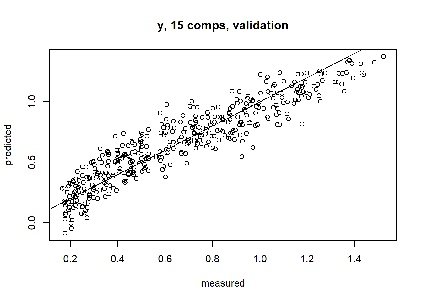
RMSEP(m1)## (Intercept) 1 comps 2 comps 3 comps 4 comps 5 comps 6 comps
## CV 0.3443 0.3103 0.2949 0.2372 0.2038 0.185 0.1824
## adjCV 0.3443 0.3103 0.2949 0.2372 0.2038 0.185 0.1824
## 7 comps 8 comps 9 comps 10 comps 11 comps 12 comps 13 comps
## CV 0.1783 0.176 0.1745 0.1659 0.1551 0.1506 0.1469
## adjCV 0.1783 0.176 0.1745 0.1659 0.1551 0.1507 0.1469
## 14 comps 15 comps
## CV 0.1351 0.1294
## adjCV 0.1351 0.1293pls::R2(m1)## (Intercept) 1 comps 2 comps 3 comps 4 comps 5 comps
## -0.005019 0.183801 0.262396 0.523111 0.647881 0.709712
## 6 comps 7 comps 8 comps 9 comps 10 comps 11 comps
## 0.717907 0.730419 0.737413 0.741790 0.766686 0.795945
## 12 comps 13 comps 14 comps 15 comps
## 0.807589 0.816953 0.845187 0.858127plot(RMSEP(m1), legendpos = "topright")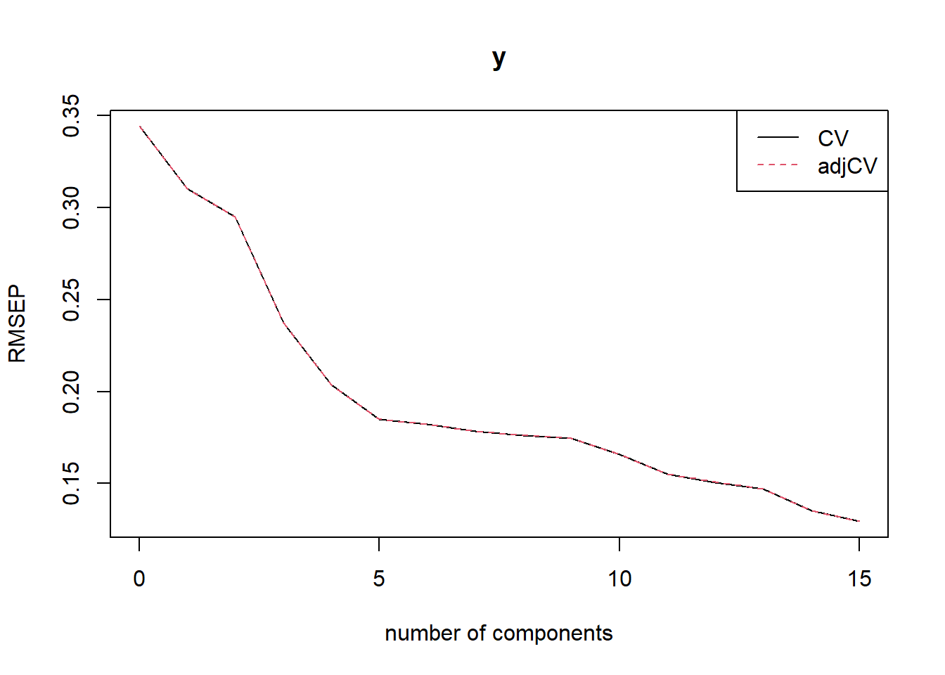
plot(m1, plottype = "scores", comps = 1:2)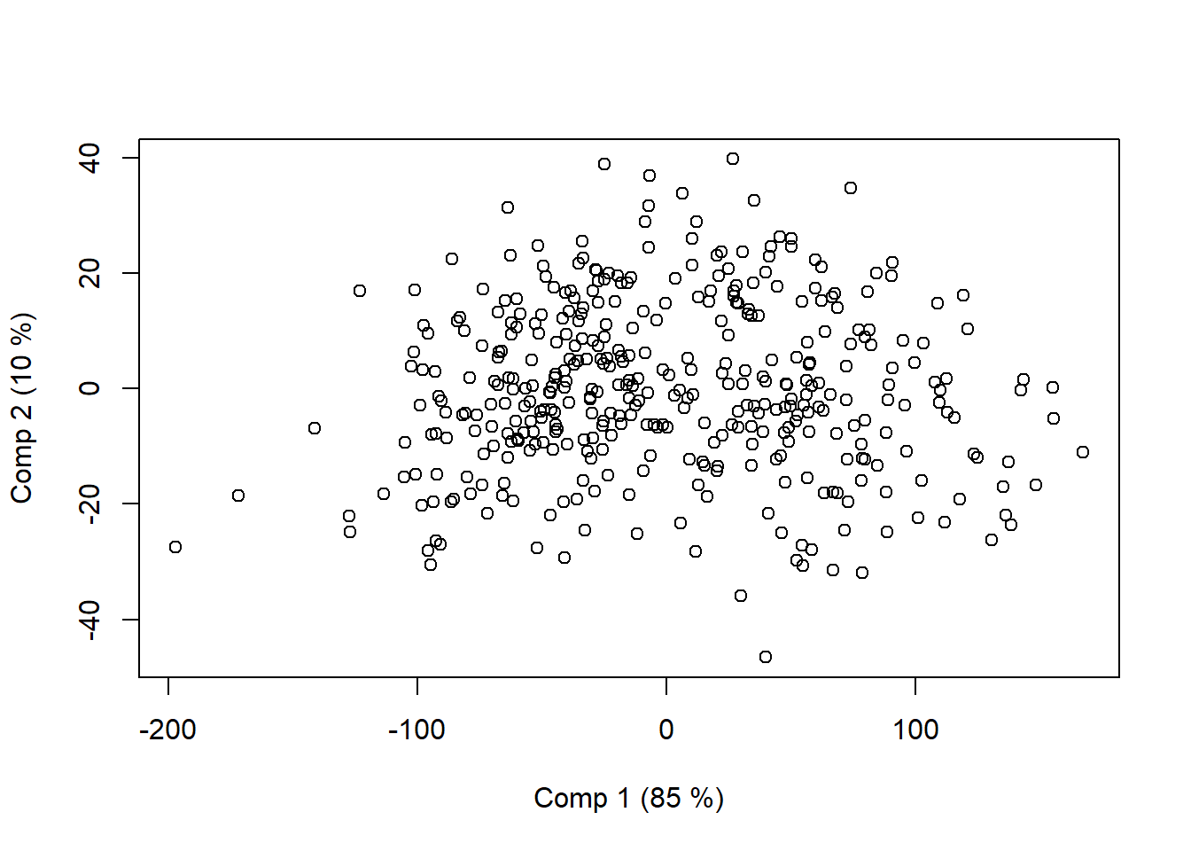
plot(m1, plottype = "loadings", comps = 1:2,legendpos = "topright")
plot(m1, plottype = "loadings", comps = 1:2,legendpos = "topright")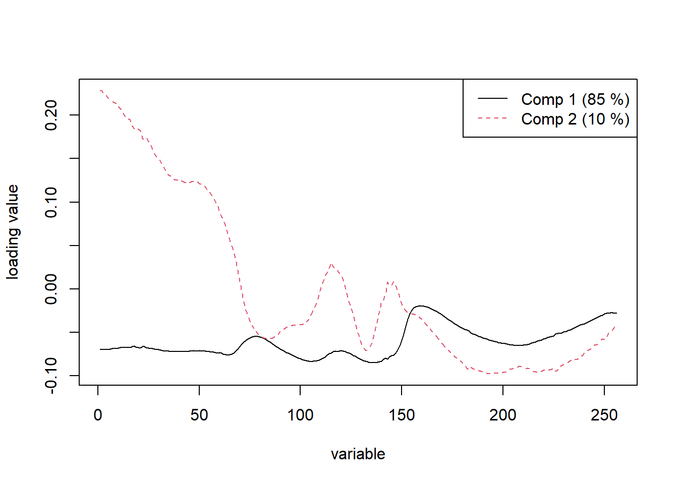
pre <- predict(m1, ncomp = 12, newdata = val)
#预测结果绘图
predplot(m1, ncomp = 12, newdata = val, asp = 1, line = TRUE)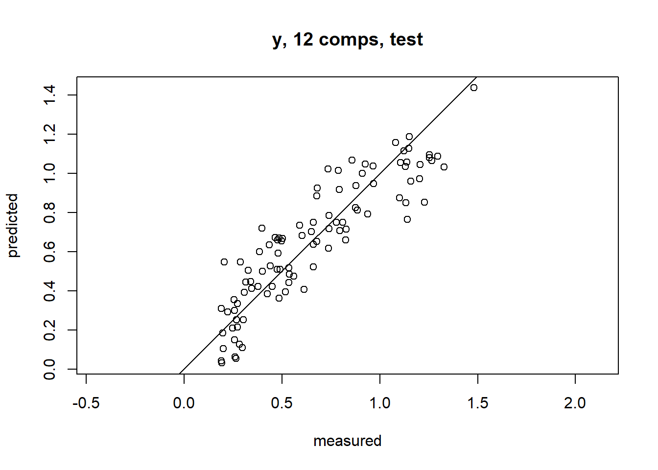
#另一种方法绘图
cbind (pre,val$y) %>% as_tibble() %>%
  rename(predicted=1,measured=2) %>%
  ggplot(aes(predicted,measured))+geom_point(size =3,col='red')+
  geom_abline(intercept = 0)+theme_classic(base_size = 13)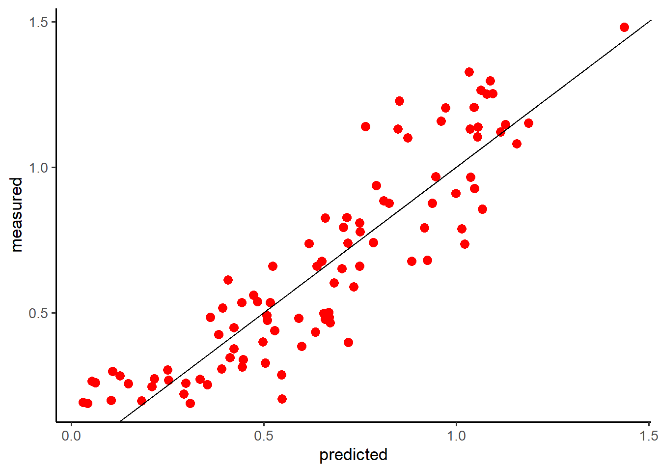
8.2.2 MLP 模型
这里我想介绍一下如何用深度学习模型进行光谱预测,要使用深度学习模型,在R里面我们通常需要安装keras安装包,可以通过以下代码进行安装,
install.packages("keras")
library(keras)
install_keras()
接下来我们用Keras来简单构建我们的光谱预测模型。首先需要要准备数据,把数据分为训练集和测试集:
library(keras)
library(pls)
library(tidyverse)
library(tfdatasets)
# library(tensorflow)
data_pls <- readRDS('data_pls.rds')
y <- data_pls$Chlo
x <- as.matrix(data_pls[,-1])
new_datapls <- cbind.data.frame(y,x)
glimpse(new_datapls)
## Rows: 497
## Columns: 257
## $ y <dbl> 0.2664, 0.2499, 0.2630, 0.4687, 0.2336, 0.1913, 0.2890, 0.444~
## $ `976.3` <dbl> 87.041, 87.682, 91.814, 86.594, 86.393, 70.167, 75.427, 81.02~
## $ `981.7` <dbl> 87.243, 87.959, 92.322, 86.870, 86.552, 70.554, 75.782, 81.37~
## $ `987.2` <dbl> 87.322, 87.997, 92.375, 86.774, 86.636, 70.581, 75.914, 81.56~
## $ `992.7` <dbl> 87.640, 88.164, 92.472, 87.054, 86.872, 70.839, 76.212, 81.76~
## $ `998.3` <dbl> 87.728, 88.416, 92.671, 87.332, 87.023, 71.003, 76.373, 81.72~
## $ `1004` <dbl> 87.869, 88.569, 92.841, 87.427, 87.319, 71.153, 76.520, 82.00~
## $ `1009.7` <dbl> 88.053, 88.809, 93.140, 87.660, 87.568, 71.517, 76.853, 82.32~
## $ `1015.5` <dbl> 88.183, 88.774, 93.256, 87.767, 87.624, 71.704, 76.995, 82.33~
## $ `1021.3` <dbl> 88.401, 89.053, 93.337, 88.002, 87.825, 71.906, 77.118, 82.49~
## $ `1027.2` <dbl> 88.703, 89.409, 93.665, 88.358, 88.115, 72.277, 77.436, 82.74~
## $ `1033.1` <dbl> 88.796, 89.389, 93.848, 88.377, 88.208, 72.430, 77.656, 82.86~
## $ `1039` <dbl> 88.971, 89.557, 93.962, 88.502, 88.372, 72.711, 77.879, 83.10~
## $ `1045` <dbl> 89.117, 89.713, 94.198, 88.725, 88.546, 72.932, 78.091, 83.28~
## $ `1051.1` <dbl> 89.291, 89.918, 94.403, 88.944, 88.706, 73.129, 78.323, 83.48~
## $ `1057.2` <dbl> 89.472, 90.075, 94.498, 89.070, 88.838, 73.387, 78.544, 83.72~
## $ `1063.2` <dbl> 89.463, 90.123, 94.431, 89.077, 88.899, 73.495, 78.609, 83.73~
## $ `1069.4` <dbl> 89.275, 89.897, 94.308, 88.984, 88.811, 73.233, 78.441, 83.58~
## $ `1075.5` <dbl> 89.354, 89.891, 94.418, 89.093, 88.959, 73.318, 78.600, 83.71~
## $ `1081.7` <dbl> 89.635, 90.188, 94.594, 89.202, 89.128, 73.713, 78.922, 84.06~
## $ `1087.9` <dbl> 89.561, 90.152, 94.526, 89.108, 89.038, 73.622, 78.885, 84.09~
## $ `1094.2` <dbl> 89.526, 90.104, 94.446, 89.090, 89.035, 73.605, 78.923, 84.08~
## $ `1100.4` <dbl> 89.314, 89.872, 94.159, 88.892, 88.874, 73.347, 78.694, 83.96~
## $ `1106.7` <dbl> 89.134, 89.739, 93.935, 88.688, 88.680, 73.102, 78.515, 83.82~
## $ `1113` <dbl> 89.024, 89.564, 93.755, 88.479, 88.561, 72.976, 78.490, 83.76~
## $ `1119.3` <dbl> 88.736, 89.310, 93.402, 88.213, 88.353, 72.592, 78.228, 83.58~
## $ `1125.6` <dbl> 88.502, 89.119, 93.122, 87.918, 88.085, 72.253, 77.974, 83.47~
## $ `1131.9` <dbl> 88.119, 88.697, 92.694, 87.470, 87.708, 71.821, 77.617, 83.19~
## $ `1138.2` <dbl> 87.662, 88.275, 92.136, 86.974, 87.325, 71.246, 77.221, 82.86~
## $ `1144.6` <dbl> 87.140, 87.778, 91.559, 86.432, 86.857, 70.620, 76.770, 82.52~
## $ `1151` <dbl> 86.713, 87.369, 91.088, 85.923, 86.377, 70.135, 76.386, 82.24~
## $ `1157.3` <dbl> 86.285, 86.960, 90.577, 85.365, 85.918, 69.572, 75.970, 81.95~
## $ `1163.7` <dbl> 85.746, 86.426, 89.937, 84.777, 85.382, 68.945, 75.452, 81.54~
## $ `1170` <dbl> 85.313, 86.000, 89.440, 84.295, 85.017, 68.448, 75.033, 81.24~
## $ `1176.4` <dbl> 84.900, 85.608, 88.982, 83.889, 84.674, 67.981, 74.649, 80.95~
## $ `1182.8` <dbl> 84.690, 85.422, 88.742, 83.643, 84.452, 67.776, 74.486, 80.77~
## $ `1189.1` <dbl> 84.619, 85.350, 88.672, 83.493, 84.350, 67.712, 74.483, 80.77~
## $ `1195.5` <dbl> 84.418, 85.158, 88.444, 83.269, 84.196, 67.520, 74.307, 80.64~
## $ `1201.9` <dbl> 84.322, 85.108, 88.370, 83.183, 84.109, 67.435, 74.252, 80.57~
## $ `1208.2` <dbl> 84.321, 85.142, 88.381, 83.162, 84.080, 67.501, 74.316, 80.61~
## $ `1214.6` <dbl> 84.309, 85.123, 88.380, 83.118, 84.073, 67.542, 74.309, 80.62~
## $ `1221` <dbl> 84.357, 85.157, 88.402, 83.138, 84.131, 67.542, 74.375, 80.65~
## $ `1227.3` <dbl> 84.389, 85.232, 88.383, 83.204, 84.144, 67.615, 74.468, 80.70~
## $ `1233.7` <dbl> 84.462, 85.306, 88.475, 83.244, 84.165, 67.756, 74.585, 80.76~
## $ `1240` <dbl> 84.485, 85.372, 88.561, 83.264, 84.220, 67.803, 74.672, 80.82~
## $ `1246.4` <dbl> 84.562, 85.522, 88.649, 83.334, 84.240, 67.968, 74.822, 80.95~
## $ `1252.7` <dbl> 84.640, 85.575, 88.685, 83.382, 84.260, 68.030, 74.921, 81.01~
## $ `1259` <dbl> 84.643, 85.542, 88.664, 83.384, 84.279, 68.016, 74.913, 80.99~
## $ `1265.3` <dbl> 84.622, 85.561, 88.609, 83.335, 84.230, 68.019, 74.915, 81.01~
## $ `1271.6` <dbl> 84.571, 85.482, 88.514, 83.226, 84.141, 67.894, 74.864, 80.94~
## $ `1277.9` <dbl> 84.423, 85.329, 88.348, 83.094, 84.028, 67.688, 74.683, 80.77~
## $ `1284.2` <dbl> 84.242, 85.178, 88.119, 82.924, 83.854, 67.533, 74.528, 80.65~
## $ `1290.5` <dbl> 83.968, 84.904, 87.787, 82.619, 83.559, 67.217, 74.238, 80.42~
## $ `1296.8` <dbl> 83.625, 84.563, 87.387, 82.255, 83.244, 66.794, 73.908, 80.14~
## $ `1303` <dbl> 83.178, 84.103, 86.871, 81.753, 82.852, 66.289, 73.441, 79.77~
## $ `1309.3` <dbl> 82.618, 83.546, 86.218, 81.159, 82.300, 65.593, 72.801, 79.25~
## $ `1315.5` <dbl> 81.953, 82.907, 85.472, 80.507, 81.682, 64.856, 72.150, 78.71~
## $ `1321.8` <dbl> 81.147, 82.114, 84.587, 79.665, 80.933, 63.986, 71.329, 78.04~
## $ `1328` <dbl> 80.393, 81.348, 83.694, 78.776, 80.118, 63.091, 70.508, 77.36~
## $ `1334.2` <dbl> 79.433, 80.390, 82.604, 77.760, 79.179, 62.045, 69.518, 76.56~
## $ `1340.4` <dbl> 78.110, 79.105, 81.162, 76.450, 77.960, 60.641, 68.182, 75.46~
## $ `1346.6` <dbl> 76.826, 77.809, 79.706, 75.074, 76.699, 59.282, 66.826, 74.33~
## $ `1352.8` <dbl> 75.494, 76.460, 78.189, 73.680, 75.382, 57.942, 65.479, 73.18~
## $ `1359` <dbl> 73.745, 74.709, 76.271, 71.915, 73.715, 56.221, 63.753, 71.67~
## $ `1365.1` <dbl> 71.830, 72.780, 74.173, 69.950, 71.849, 54.410, 61.848, 70.01~
## $ `1371.3` <dbl> 69.694, 70.629, 71.852, 67.786, 69.751, 52.440, 59.732, 68.10~
## $ `1377.4` <dbl> 67.203, 68.116, 69.139, 65.286, 67.358, 50.193, 57.264, 65.88~
## $ `1383.5` <dbl> 64.329, 65.213, 65.997, 62.440, 64.637, 47.625, 54.426, 63.31~
## $ `1389.7` <dbl> 60.975, 61.805, 62.382, 59.164, 61.414, 44.779, 51.220, 60.36~
## $ `1395.8` <dbl> 57.177, 57.974, 58.326, 55.444, 57.723, 41.676, 47.688, 57.08~
## $ `1401.9` <dbl> 52.870, 53.701, 53.786, 51.231, 53.604, 38.265, 43.740, 53.37~
## $ `1408` <dbl> 48.467, 49.349, 49.237, 46.938, 49.324, 34.947, 39.833, 49.55~
## $ `1414` <dbl> 44.233, 45.165, 44.924, 42.852, 45.229, 31.778, 36.163, 45.85~
## $ `1420.1` <dbl> 40.440, 41.439, 41.078, 39.175, 41.556, 28.985, 32.871, 42.48~
## $ `1426.2` <dbl> 37.455, 38.558, 38.137, 36.273, 38.658, 26.902, 30.346, 39.83~
## $ `1432.2` <dbl> 35.058, 36.273, 35.827, 34.011, 36.369, 25.195, 28.369, 37.71~
## $ `1438.3` <dbl> 33.302, 34.588, 34.140, 32.343, 34.697, 23.957, 26.908, 36.15~
## $ `1444.3` <dbl> 32.275, 33.653, 33.192, 31.294, 33.695, 23.274, 26.087, 35.23~
## $ `1450.4` <dbl> 31.632, 33.094, 32.648, 30.702, 33.113, 22.830, 25.595, 34.68~
## $ `1456.4` <dbl> 31.355, 32.897, 32.475, 30.491, 32.913, 22.668, 25.411, 34.50~
## $ `1462.4` <dbl> 31.419, 33.053, 32.654, 30.592, 33.027, 22.751, 25.519, 34.63~
## $ `1468.4` <dbl> 31.686, 33.415, 33.029, 30.876, 33.355, 22.951, 25.791, 34.93~
## $ `1474.4` <dbl> 32.307, 34.108, 33.728, 31.465, 33.999, 23.406, 26.340, 35.56~
## $ `1480.4` <dbl> 33.171, 35.008, 34.678, 32.310, 34.898, 24.016, 27.059, 36.41~
## $ `1486.4` <dbl> 34.272, 36.166, 35.859, 33.370, 36.002, 24.824, 28.013, 37.44~
## $ `1492.4` <dbl> 35.497, 37.425, 37.162, 34.573, 37.228, 25.679, 29.041, 38.56~
## $ `1498.4` <dbl> 36.820, 38.778, 38.576, 35.839, 38.585, 26.564, 30.155, 39.78~
## $ `1504.3` <dbl> 38.430, 40.447, 40.271, 37.342, 40.144, 27.746, 31.536, 41.28~
## $ `1510.3` <dbl> 39.949, 42.006, 41.884, 38.813, 41.653, 28.811, 32.796, 42.61~
## $ `1516.2` <dbl> 41.481, 43.547, 43.512, 40.274, 43.188, 29.888, 34.073, 43.97~
## $ `1522.2` <dbl> 43.071, 45.178, 45.222, 41.808, 44.744, 31.061, 35.434, 45.40~
## $ `1528.2` <dbl> 44.548, 46.656, 46.748, 43.226, 46.201, 32.024, 36.658, 46.67~
## $ `1534.1` <dbl> 46.089, 48.191, 48.323, 44.666, 47.701, 33.115, 37.924, 47.97~
## $ `1540.1` <dbl> 47.540, 49.668, 49.854, 46.037, 49.100, 34.197, 39.180, 49.20~
## $ `1546` <dbl> 48.898, 51.018, 51.276, 47.321, 50.414, 35.166, 40.346, 50.36~
## $ `1551.9` <dbl> 50.142, 52.236, 52.587, 48.527, 51.656, 36.038, 41.366, 51.39~
## $ `1557.9` <dbl> 51.403, 53.469, 53.879, 49.714, 52.876, 36.932, 42.409, 52.42~
## $ `1563.8` <dbl> 52.620, 54.669, 55.144, 50.878, 54.037, 37.813, 43.428, 53.40~
## $ `1569.8` <dbl> 53.729, 55.730, 56.273, 51.934, 55.111, 38.581, 44.318, 54.23~
## $ `1575.7` <dbl> 54.789, 56.782, 57.376, 52.936, 56.155, 39.338, 45.189, 55.09~
## $ `1581.6` <dbl> 55.745, 57.730, 58.383, 53.853, 57.074, 39.979, 45.955, 55.83~
## $ `1587.5` <dbl> 56.632, 58.581, 59.280, 54.704, 57.949, 40.583, 46.644, 56.43~
## $ `1593.5` <dbl> 57.508, 59.417, 60.205, 55.556, 58.784, 41.187, 47.303, 57.07~
## $ `1599.4` <dbl> 58.284, 60.177, 60.998, 56.308, 59.540, 41.642, 47.906, 57.63~
## $ `1605.3` <dbl> 59.048, 60.939, 61.799, 57.044, 60.309, 42.186, 48.532, 58.20~
## $ `1611.2` <dbl> 59.923, 61.723, 62.646, 57.854, 61.090, 42.812, 49.184, 58.84~
## $ `1617.2` <dbl> 60.540, 62.268, 63.216, 58.508, 61.724, 43.137, 49.543, 59.21~
## $ `1623.1` <dbl> 61.186, 62.878, 63.900, 59.174, 62.382, 43.559, 50.009, 59.65~
## $ `1629` <dbl> 61.808, 63.417, 64.524, 59.768, 63.017, 43.922, 50.407, 60.05~
## $ `1635` <dbl> 62.319, 63.877, 65.009, 60.327, 63.581, 44.228, 50.690, 60.38~
## $ `1640.9` <dbl> 62.924, 64.431, 65.594, 60.963, 64.134, 44.693, 51.166, 60.85~
## $ `1646.8` <dbl> 63.429, 64.817, 66.056, 61.430, 64.576, 44.980, 51.441, 61.15~
## $ `1652.8` <dbl> 63.859, 65.189, 66.475, 61.851, 65.019, 45.312, 51.748, 61.47~
## $ `1658.7` <dbl> 64.057, 65.368, 66.700, 62.132, 65.292, 45.420, 51.874, 61.67~
## $ `1664.6` <dbl> 64.243, 65.523, 66.890, 62.338, 65.484, 45.559, 51.985, 61.85~
## $ `1670.6` <dbl> 64.538, 65.755, 67.145, 62.580, 65.704, 45.930, 52.302, 62.19~
## $ `1676.5` <dbl> 64.478, 65.621, 67.068, 62.569, 65.720, 45.883, 52.239, 62.13~
## $ `1682.5` <dbl> 64.429, 65.574, 67.041, 62.505, 65.750, 45.948, 52.274, 62.14~
## $ `1688.4` <dbl> 64.326, 65.493, 66.973, 62.367, 65.667, 45.969, 52.272, 62.07~
## $ `1694.4` <dbl> 64.018, 65.135, 66.687, 62.067, 65.397, 45.753, 52.030, 61.75~
## $ `1700.3` <dbl> 63.728, 64.840, 66.443, 61.737, 65.125, 45.660, 51.905, 61.57~
## $ `1706.3` <dbl> 63.351, 64.490, 66.079, 61.311, 64.752, 45.438, 51.659, 61.31~
## $ `1712.2` <dbl> 62.916, 64.093, 65.670, 60.840, 64.325, 45.223, 51.438, 61.07~
## $ `1718.2` <dbl> 62.376, 63.578, 65.167, 60.271, 63.798, 44.967, 51.136, 60.76~
## $ `1724.2` <dbl> 61.820, 63.057, 64.634, 59.743, 63.278, 44.637, 50.773, 60.38~
## $ `1730.2` <dbl> 61.286, 62.588, 64.122, 59.225, 62.738, 44.366, 50.510, 60.09~
## $ `1736.1` <dbl> 60.737, 62.087, 63.527, 58.658, 62.137, 44.088, 50.177, 59.78~
## $ `1742.1` <dbl> 60.063, 61.445, 62.846, 58.039, 61.492, 43.608, 49.690, 59.32~
## $ `1748.1` <dbl> 59.395, 60.831, 62.166, 57.371, 60.806, 43.136, 49.220, 58.88~
## $ `1754.1` <dbl> 58.734, 60.249, 61.460, 56.677, 60.081, 42.580, 48.644, 58.28~
## $ `1760.1` <dbl> 57.850, 59.448, 60.562, 55.922, 59.261, 41.821, 47.832, 57.49~
## $ `1766.1` <dbl> 57.167, 58.780, 59.840, 55.243, 58.554, 41.251, 47.210, 56.90~
## $ `1772.1` <dbl> 56.518, 58.143, 59.128, 54.588, 57.905, 40.584, 46.536, 56.27~
## $ `1778.1` <dbl> 55.866, 57.529, 58.434, 54.046, 57.306, 39.984, 45.896, 55.65~
## $ `1784.1` <dbl> 55.459, 57.134, 57.965, 53.612, 56.844, 39.558, 45.481, 55.21~
## $ `1790.1` <dbl> 55.040, 56.712, 57.475, 53.237, 56.437, 38.986, 44.968, 54.74~
## $ `1796.1` <dbl> 54.802, 56.484, 57.175, 53.038, 56.177, 38.696, 44.631, 54.44~
## $ `1802.1` <dbl> 54.652, 56.299, 56.979, 52.880, 55.993, 38.390, 44.348, 54.16~
## $ `1808.2` <dbl> 54.494, 56.109, 56.706, 52.768, 55.866, 38.022, 44.060, 53.83~
## $ `1814.2` <dbl> 54.420, 55.992, 56.539, 52.668, 55.792, 37.788, 43.867, 53.59~
## $ `1820.2` <dbl> 54.401, 55.957, 56.537, 52.602, 55.673, 37.664, 43.775, 53.55~
## $ `1826.3` <dbl> 54.058, 55.636, 56.149, 52.328, 55.378, 37.249, 43.391, 53.18~
## $ `1832.3` <dbl> 53.715, 55.224, 55.700, 51.968, 55.064, 36.844, 43.011, 52.85~
## $ `1838.4` <dbl> 53.391, 54.865, 55.337, 51.573, 54.584, 36.659, 42.759, 52.54~
## $ `1844.4` <dbl> 52.390, 53.882, 54.258, 50.687, 53.668, 35.812, 41.879, 51.64~
## $ `1850.5` <dbl> 51.205, 52.685, 52.936, 49.484, 52.486, 34.887, 40.880, 50.63~
## $ `1856.5` <dbl> 49.591, 51.031, 51.215, 47.859, 50.764, 33.764, 39.554, 49.23~
## $ `1862.6` <dbl> 47.026, 48.435, 48.449, 45.388, 48.229, 31.852, 37.378, 47.03~
## $ `1868.6` <dbl> 43.650, 45.054, 44.907, 42.089, 44.878, 29.504, 34.602, 44.16~
## $ `1874.7` <dbl> 39.193, 40.556, 40.286, 37.826, 40.465, 26.418, 30.937, 40.23~
## $ `1880.8` <dbl> 33.743, 35.007, 34.614, 32.560, 35.039, 22.644, 26.451, 35.27~
## $ `1886.8` <dbl> 27.887, 29.048, 28.645, 26.868, 29.187, 18.744, 21.780, 29.94~
## $ `1892.9` <dbl> 22.082, 23.116, 22.753, 21.252, 23.317, 14.932, 17.213, 24.43~
## $ `1899` <dbl> 17.240, 18.152, 17.906, 16.594, 18.440, 11.794, 13.448, 19.64~
## $ `1905.1` <dbl> 13.923, 14.743, 14.626, 13.384, 15.081, 9.687, 10.919, 16.281~
## $ `1911.2` <dbl> 11.807, 12.530, 12.538, 11.257, 12.832, 8.283, 9.284, 13.992,~
## $ `1917.2` <dbl> 10.413, 11.062, 11.254, 9.885, 11.408, 7.360, 8.231, 12.516, ~
## $ `1923.3` <dbl> 9.518, 10.174, 10.381, 9.066, 10.517, 6.803, 7.563, 11.649, 1~
## $ `1929.4` <dbl> 9.029, 9.633, 9.839, 8.541, 9.960, 6.453, 7.152, 11.092, 9.54~
## $ `1935.5` <dbl> 8.642, 9.291, 9.526, 8.182, 9.647, 6.213, 6.863, 10.780, 9.19~
## $ `1941.6` <dbl> 8.426, 9.130, 9.389, 8.048, 9.560, 6.128, 6.711, 10.677, 9.04~
## $ `1947.7` <dbl> 8.383, 9.077, 9.346, 8.011, 9.481, 6.091, 6.653, 10.719, 9.02~
## $ `1953.8` <dbl> 8.502, 9.257, 9.459, 8.110, 9.636, 6.168, 6.721, 10.910, 9.15~
## $ `1959.8` <dbl> 8.749, 9.589, 9.754, 8.397, 9.984, 6.351, 6.936, 11.276, 9.46~
## $ `1965.9` <dbl> 9.092, 9.978, 10.115, 8.737, 10.388, 6.620, 7.188, 11.774, 9.~
## $ `1972` <dbl> 9.539, 10.507, 10.645, 9.217, 10.947, 6.977, 7.547, 12.397, 1~
## $ `1978.1` <dbl> 10.078, 11.127, 11.268, 9.790, 11.584, 7.343, 8.011, 13.139, ~
## $ `1984.2` <dbl> 10.769, 11.817, 11.929, 10.462, 12.310, 7.746, 8.458, 13.872,~
## $ `1990.3` <dbl> 11.472, 12.607, 12.680, 11.179, 13.054, 8.223, 9.030, 14.754,~
## $ `1996.4` <dbl> 12.237, 13.484, 13.517, 11.971, 13.935, 8.816, 9.686, 15.679,~
## $ `2002.5` <dbl> 13.048, 14.333, 14.393, 12.786, 14.883, 9.411, 10.275, 16.549~
## $ `2008.5` <dbl> 13.908, 15.266, 15.275, 13.626, 15.806, 10.009, 11.011, 17.59~
## $ `2014.6` <dbl> 14.771, 16.181, 16.224, 14.499, 16.736, 10.608, 11.735, 18.53~
## $ `2020.7` <dbl> 15.720, 17.196, 17.241, 15.413, 17.727, 11.276, 12.442, 19.50~
## $ `2026.8` <dbl> 16.583, 18.168, 18.141, 16.269, 18.658, 11.897, 13.125, 20.47~
## $ `2032.9` <dbl> 17.471, 19.041, 19.051, 17.139, 19.617, 12.493, 13.845, 21.38~
## $ `2038.9` <dbl> 18.371, 19.944, 20.047, 17.990, 20.549, 13.144, 14.534, 22.24~
## $ `2045` <dbl> 19.133, 20.842, 20.889, 18.724, 21.351, 13.740, 15.195, 23.10~
## $ `2051.1` <dbl> 19.996, 21.684, 21.733, 19.571, 22.258, 14.316, 15.889, 23.95~
## $ `2057.1` <dbl> 20.867, 22.556, 22.694, 20.401, 23.143, 14.950, 16.551, 24.73~
## $ `2063.2` <dbl> 21.682, 23.359, 23.549, 21.092, 23.956, 15.517, 17.210, 25.54~
## $ `2069.2` <dbl> 22.491, 24.215, 24.438, 21.868, 24.811, 16.134, 17.875, 26.35~
## $ `2075.3` <dbl> 23.140, 24.973, 25.199, 22.585, 25.577, 16.605, 18.435, 27.03~
## $ `2081.3` <dbl> 23.947, 25.742, 26.034, 23.347, 26.402, 17.194, 19.119, 27.86~
## $ `2087.4` <dbl> 24.884, 26.681, 26.935, 24.160, 27.255, 17.926, 19.857, 28.65~
## $ `2093.4` <dbl> 25.613, 27.429, 27.665, 24.828, 27.967, 18.451, 20.406, 29.35~
## $ `2099.4` <dbl> 26.368, 28.203, 28.509, 25.566, 28.756, 19.011, 21.096, 30.08~
## $ `2105.5` <dbl> 27.129, 28.971, 29.337, 26.275, 29.498, 19.558, 21.690, 30.75~
## $ `2111.5` <dbl> 27.845, 29.747, 30.085, 26.958, 30.251, 20.127, 22.307, 31.53~
## $ `2117.5` <dbl> 28.566, 30.456, 30.811, 27.631, 30.997, 20.656, 22.927, 32.24~
## $ `2123.5` <dbl> 29.248, 31.112, 31.532, 28.246, 31.666, 21.140, 23.459, 32.88~
## $ `2129.5` <dbl> 29.849, 31.744, 32.218, 28.858, 32.245, 21.613, 23.978, 33.49~
## $ `2135.5` <dbl> 30.417, 32.336, 32.843, 29.385, 32.819, 22.018, 24.449, 34.01~
## $ `2141.5` <dbl> 30.989, 32.927, 33.430, 29.962, 33.445, 22.431, 24.929, 34.54~
## $ `2147.5` <dbl> 31.552, 33.517, 33.989, 30.473, 33.966, 22.895, 25.412, 35.10~
## $ `2153.5` <dbl> 32.030, 34.047, 34.577, 30.930, 34.488, 23.172, 25.828, 35.57~
## $ `2159.5` <dbl> 32.488, 34.420, 35.021, 31.326, 34.980, 23.376, 26.123, 35.95~
## $ `2165.4` <dbl> 32.916, 34.848, 35.367, 31.704, 35.436, 23.760, 26.512, 36.41~
## $ `2171.4` <dbl> 33.363, 35.308, 35.886, 32.167, 35.919, 24.120, 26.998, 36.78~
## $ `2177.4` <dbl> 33.802, 35.680, 36.240, 32.543, 36.210, 24.352, 27.226, 37.05~
## $ `2183.3` <dbl> 34.165, 36.077, 36.565, 32.876, 36.607, 24.510, 27.496, 37.42~
## $ `2189.3` <dbl> 34.410, 36.299, 36.882, 33.150, 36.913, 24.635, 27.783, 37.68~
## $ `2195.2` <dbl> 34.787, 36.550, 37.161, 33.420, 37.181, 24.856, 28.071, 38.07~
## $ `2201.2` <dbl> 35.041, 36.867, 37.432, 33.740, 37.476, 25.044, 28.317, 38.43~
## $ `2207.1` <dbl> 35.156, 37.055, 37.527, 33.883, 37.758, 25.175, 28.527, 38.60~
## $ `2213.1` <dbl> 35.405, 37.241, 37.704, 34.032, 37.899, 25.328, 28.785, 38.83~
## $ `2219` <dbl> 35.514, 37.291, 37.778, 34.165, 37.877, 25.263, 28.822, 38.90~
## $ `2224.9` <dbl> 35.543, 37.319, 37.770, 34.159, 38.033, 25.198, 28.688, 38.81~
## $ `2230.8` <dbl> 35.471, 37.264, 37.728, 34.118, 37.885, 25.184, 28.669, 38.72~
## $ `2236.8` <dbl> 35.182, 36.994, 37.455, 33.921, 37.665, 24.963, 28.524, 38.55~
## $ `2242.7` <dbl> 34.842, 36.678, 37.112, 33.545, 37.420, 24.741, 28.207, 38.23~
## $ `2248.6` <dbl> 34.308, 36.066, 36.635, 33.028, 36.929, 24.424, 27.814, 37.69~
## $ `2254.5` <dbl> 33.802, 35.539, 36.129, 32.558, 36.433, 24.079, 27.368, 37.14~
## $ `2260.4` <dbl> 33.333, 35.007, 35.656, 31.925, 35.789, 23.797, 26.950, 36.54~
## $ `2266.3` <dbl> 32.600, 34.217, 34.885, 31.051, 35.127, 23.229, 26.365, 35.76~
## $ `2272.3` <dbl> 31.889, 33.534, 34.203, 30.412, 34.442, 22.674, 25.743, 35.08~
## $ `2278.2` <dbl> 31.228, 32.885, 33.686, 29.879, 33.828, 22.362, 25.062, 34.35~
## $ `2284.1` <dbl> 30.667, 32.319, 33.145, 29.250, 33.345, 21.982, 24.595, 33.77~
## $ `2290` <dbl> 30.147, 31.728, 32.538, 28.651, 32.752, 21.494, 24.172, 33.26~
## $ `2295.9` <dbl> 29.397, 31.070, 31.886, 28.095, 32.139, 20.981, 23.578, 32.55~
## $ `2301.8` <dbl> 28.833, 30.369, 31.147, 27.376, 31.372, 20.526, 23.060, 31.90~
## $ `2307.8` <dbl> 28.149, 29.586, 30.391, 26.671, 30.679, 20.009, 22.416, 31.13~
## $ `2313.7` <dbl> 27.401, 28.973, 29.759, 26.131, 30.076, 19.585, 21.836, 30.52~
## $ `2319.6` <dbl> 26.979, 28.546, 29.237, 25.594, 29.604, 19.312, 21.554, 30.22~
## $ `2325.6` <dbl> 26.393, 27.985, 28.697, 25.059, 29.034, 18.836, 21.084, 29.81~
## $ `2331.5` <dbl> 25.904, 27.525, 28.040, 24.582, 28.407, 18.486, 20.567, 29.29~
## $ `2337.5` <dbl> 25.354, 26.858, 27.495, 23.967, 27.944, 17.985, 20.170, 28.71~
## $ `2343.5` <dbl> 24.676, 26.128, 26.867, 23.255, 27.155, 17.641, 19.673, 28.23~
## $ `2349.5` <dbl> 24.017, 25.546, 26.228, 22.988, 26.402, 17.322, 19.111, 27.78~
## $ `2355.5` <dbl> 23.434, 25.013, 25.605, 22.431, 25.995, 16.694, 18.578, 27.10~
## $ `2361.5` <dbl> 23.042, 24.464, 24.871, 21.724, 25.360, 16.355, 18.164, 26.46~
## $ `2367.5` <dbl> 22.366, 23.807, 24.228, 21.204, 24.720, 15.958, 17.801, 26.05~
## $ `2373.5` <dbl> 21.825, 23.228, 23.696, 20.596, 24.214, 15.548, 17.284, 25.59~
## $ `2379.6` <dbl> 21.268, 22.723, 23.014, 20.169, 23.590, 15.113, 16.671, 24.85~
## $ `2385.7` <dbl> 20.581, 22.123, 22.358, 19.576, 22.856, 14.630, 16.247, 24.33~
## $ `2391.8` <dbl> 20.157, 21.345, 21.764, 18.924, 22.186, 14.253, 15.782, 23.75~
## $ `2397.9` <dbl> 19.419, 20.694, 21.095, 18.238, 21.569, 13.569, 15.019, 22.99~
## $ `2404.1` <dbl> 18.627, 20.207, 20.395, 17.675, 20.888, 13.145, 14.698, 22.42~
## $ `2410.3` <dbl> 18.271, 19.520, 19.832, 17.178, 20.325, 13.013, 14.293, 21.86~
## $ `2416.5` <dbl> 17.645, 18.702, 19.312, 16.588, 19.565, 12.432, 13.622, 21.26~
## $ `2422.7` <dbl> 16.955, 18.266, 18.562, 15.995, 18.994, 12.027, 13.132, 20.88~
## $ `2429` <dbl> 16.558, 17.662, 18.060, 15.442, 18.477, 11.775, 12.717, 20.13~
## $ `2435.3` <dbl> 15.904, 17.004, 17.692, 14.876, 17.713, 11.367, 12.424, 19.20~
## $ `2441.7` <dbl> 15.219, 16.508, 16.698, 14.286, 17.146, 10.772, 11.855, 18.79~
## $ `2448.1` <dbl> 14.842, 15.934, 15.984, 13.672, 16.495, 10.457, 11.259, 18.16~
## $ `2454.5` <dbl> 14.288, 15.220, 15.634, 12.898, 15.674, 10.216, 11.109, 17.49~
## $ `2461` <dbl> 13.728, 14.709, 15.145, 12.888, 15.488, 9.540, 10.716, 16.942~
## $ `2467.5` <dbl> 13.422, 14.328, 14.781, 12.297, 14.985, 9.162, 10.180, 16.253~
## $ `2474.1` <dbl> 12.931, 13.867, 14.160, 11.568, 14.331, 8.946, 9.912, 16.149,~
## $ `2480.7` <dbl> 12.316, 13.235, 13.542, 11.415, 14.103, 8.878, 9.631, 15.564,~
## $ `2487.4` <dbl> 11.778, 12.739, 13.123, 10.901, 13.630, 8.592, 9.158, 14.659,~
## $ `2494.1` <dbl> 11.739, 12.414, 13.089, 10.718, 12.954, 8.336, 8.953, 14.641,~
## $ `2500.9` <dbl> 11.743, 12.312, 13.024, 10.655, 12.701, 8.667, 9.177, 14.519,~
## $ `2507.8` <dbl> 11.370, 12.349, 12.575, 10.241, 12.790, 8.233, 8.859, 14.458,~
## $ `2514.8` <dbl> 11.391, 12.199, 12.441, 10.064, 12.827, 8.043, 8.744, 14.219,~
## $ `2521.8` <dbl> 11.930, 12.195, 12.725, 10.402, 12.616, 8.091, 8.733, 14.227,~
## $ `2528.8` <dbl> 12.230, 11.952, 13.064, 10.801, 12.316, 7.330, 8.459, 14.639,~library(caTools)
set.seed(123) # set seed to ensure you always have same random numbers generated
sample = sample.split(new_datapls,SplitRatio = 0.60) # splits the data in the ratio mentioned in SplitRatio. After splitting Decks these rows as logical TRUE and the the remaining are marked as logical FALSE
train1 =subset(new_datapls,sample ==TRUE) # creates a training dataset named train1 with rows which are marked as TRUE
test1=subset(new_datapls, sample==FALSE)
library(dplyr)
trainy <- as.matrix(train1$y)
testy <- as.matrix(test1$y)
trainx <- as.matrix(train1[,-1])
testx <- as.matrix( test1[,-1])
summary(trainy)## V1
## Min. :0.1722
## 1st Qu.:0.3848
## Median :0.6554
## Mean :0.6654
## 3rd Qu.:0.8962
## Max. :1.4830dim(testx)## [1] 199 256model = keras_model_sequential() %>%
layer_dense(units=64, activation="relu", input_shape=256) %>%
layer_dense(units=32, activation = "relu", kernel_regularizer = regularizer_l2( 1e-04)) %>%
layer_dense(units=16, activation = "relu") %>%
layer_dense(units=1, activation="linear")
model %>% compile(
loss = "mse",
optimizer = "adam",
metrics = list("mean_absolute_error")
)
model %>% summary()## Model: "sequential"
## ________________________________________________________________________________
## Layer (type) Output Shape Param #
## ================================================================================
## dense_3 (Dense) (None, 64) 16448
## ________________________________________________________________________________
## dense_2 (Dense) (None, 32) 2080
## ________________________________________________________________________________
## dense_1 (Dense) (None, 16) 528
## ________________________________________________________________________________
## dense (Dense) (None, 1) 17
## ================================================================================
## Total params: 19,073
## Trainable params: 19,073
## Non-trainable params: 0
## ________________________________________________________________________________history <- model %>% fit(trainx, trainy, epochs = 200,verbose = 1)
plot(history)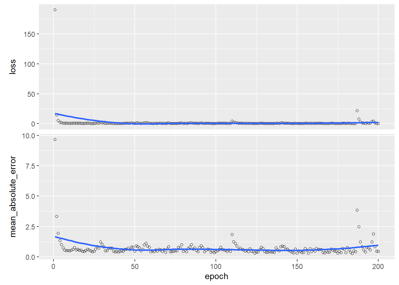
scores = model %>% evaluate(trainx, trainy, verbose = 1)
print(scores)
## loss mean_absolute_error
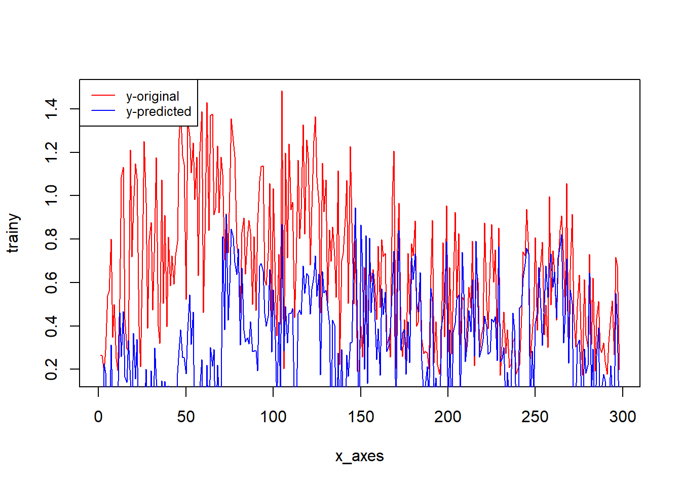
## 0.2414916 0.3848826y_pred = model %>% predict(trainx)
x_axes = seq(1:length(y_pred))
plot(x_axes, trainy, type="l", col="red")
lines(x_axes, y_pred, col="blue")
legend("topleft", legend=c("y-original", "y-predicted"),
col=c("red", "blue"), lty=1,cex=0.8)