VaR and Expected Shortfall
Exercise question
We consider daily losses on a position in a particular stock; the current value of the position equals \(V_t = 10 000\). Recall that the loss for this portfolio is given by \[ L^{\Delta}_{t+1} = -V_t \omega_t^\prime X_{t+1}, \] where \(X_{t+1}\) represents daily log-returns of the stock. We assume that \(X_{t+1}\) has mean zero and standard deviation \(\sigma = 0.2/\sqrt{250}\), i.e. we assume that the stock has an annualised volatility of \(20\%\).
We compare two different models for the distribution, namely
a normal distribution; and
a \(t\)-distribution with \(\nu=4\) degrees of freedom scaled to have standard deviation \(\sigma\).
- For a standard \(t\)-distribution \(t(\nu, 0, 1)\), the variance is \(\frac{\nu}{\nu-2}\).
- The \(t\)-distribution is a symmetric distribution with heavy tails, so that large absolute values are much more probable than in the normal model; it is also a distribution that has been shown to fit well in many empirical studies.
Evaluate and present in table of \(\text{VaR}_\alpha\) and \(\text{ES}_\alpha\) for both models and various values of \(\alpha \in (0.9,1)\).
Compare your \(\text{VaR}_\alpha\) with \(\text{ES}_\alpha\). What findings/conclusions can you draw from your comparisons?
Reference codes
First of all, before compiling our scripts, we clean all objects from memory.
The ls() code lists all of the objects in your workspace. The rm() code removes objects in your workspace. You can begin your code with the rm() function to clear all of the objects from your workspace to start with a clean environment. This way the workspace is empty and everything you create is clearly visible.
There are basically two extremely important functions when it comes down to R packages:
install.packages("package"), which as you can expect, installs a given package.library("package")which loads packages, i.e. attaches them to the search list on your R workspace.
In this exercise, we will need to load the QRM and/or qrmtools package, comprehensive packages for modelling and managing risk.
- Set parameters.
Define a set of quantile probabilities p; and the corresponding alpha-type probabilities for the upper tail. Both sets are vectors.
Further, we define the daily standard deviation and the degree of freedom.
# Standard deviation (daily)
sigma <- 0.2*10000/sqrt(250)
# Degrees of freedom when using the Student t distribution
t.dof <- 4- VaR based on the normal distribution.
As p is a vector of quantiles, plugging it into the inverse normal quantile function results in a vector of VaRs.
We get the same results using the (upper tail) alpha vector if we specify lower.tail=FALSE.
- VaR using the student t distribution.
Note: in the package QRM, this can be done by calling qst(p,mu=0,sd=sigma,df=t.dof,scale=TRUE). See ?qst for full details.
- Expected shortfall based on the normal distribution.
For a given p, the expected loss given a loss exceeds the corresponding VaR is obtained by:
The function ESnorm returns the expected loss given a loss exceeding p under normality, scaled by sigma. The expected loss is calculated by integrating over the tail of the normal distribution, dividing by its length and multiplying by sigma: sd * dnorm(qnorm(p))/(1 - p). See ?ESnorm for full details.
- Expected shortfall using student t.
This function is similar to the above. However, while using the t distribution, scaling is necessary to adjust for the degrees of freedom. Therefore, we set scale=TRUE when calling the function. See ?ESst for full details.
- Shortfall-to-quantile ratio.
## [1] 1.369421 1.254040 1.192778 1.145665 1.122725 1.089591 1.064389 1.050140 1.041004## [1] 1.630140 1.502392 1.438371 1.393290 1.373740 1.350338 1.338540 1.334964 1.333847- Display the comparisons in a matrix and two figures.
##              p VaR.normal    VaR.t4 ES.normal     ES.t4 Ratio.normal Ratio.t4
##  [1,] 0.900000   162.1049  137.1341  221.9898  223.5478     1.369421 1.630140
##  [2,] 0.950000   208.0594  190.6782  260.9148  286.4734     1.254040 1.502392
##  [3,] 0.975000   247.9180  248.3328  295.7113  357.1946     1.192778 1.438371
##  [4,] 0.990000   294.2623  335.1372  337.1259  466.9432     1.145665 1.393290
##  [5,] 0.995000   325.8195  411.8028  365.8058  565.7101     1.122725 1.373740
##  [6,] 0.999000   390.8869  641.5889  425.9069  866.3618     1.089591 1.350338
##  [7,] 0.999900   470.4225 1165.7670  500.7125 1560.4264     1.064389 1.338540
##  [8,] 0.999990   539.4708 2086.8939  566.5199 2785.9275     1.050140 1.334964
## [9,] 0.999999 601.2659 3718.8363 625.9201 4960.3597 1.041004 1.333847plot(p,VaR.normal,type="o",ylim=c(min(summary[,2:5]),max(summary[,2:5])),ylab="")
title("VaR and Expected Shortfall")
lines(p,VaR.t4,type="o",col=2)
lines(p,ES.normal,type="o",col=3)
lines(p,ES.t4,type="o",col=4)
legend.names <- c("VaR, normal", "VaR, t", "VaR, normal", "ES, t")
legend("topleft", legend = legend.names, col=1:4, pch=1)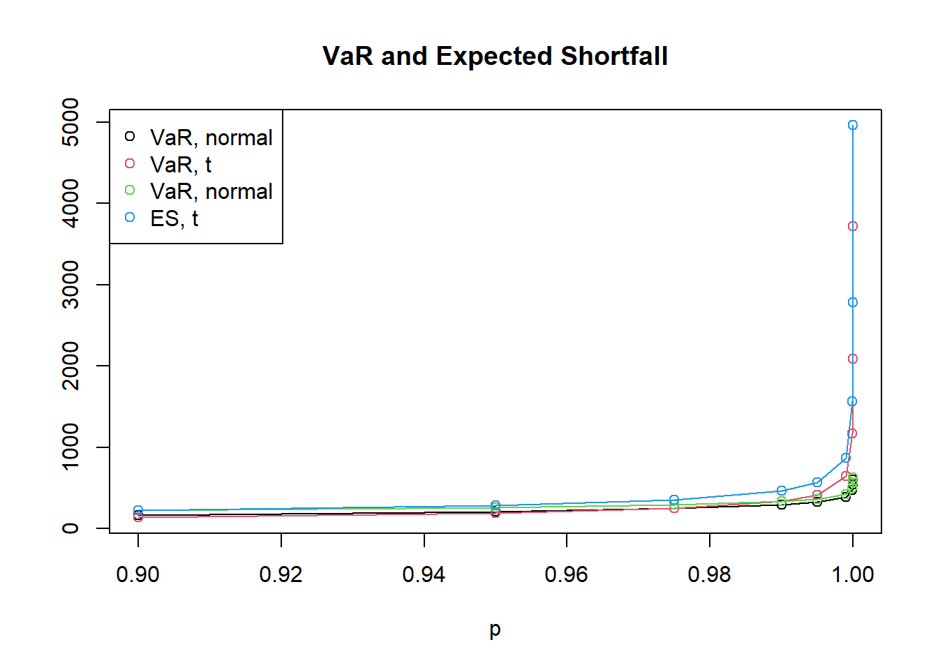
plot(p,Ratio.normal,type="o",ylim=c(min(summary[,6:7]),max(summary[,6:7])),ylab="")
title("Shortfall-to-Quantile ratio")
lines(p,Ratio.t4,type="o",col=2)
legend.names <- c("ES/VaR, normal", "ES/VaR, t")
legend("bottomleft", legend = legend.names, col=1:4, pch=1)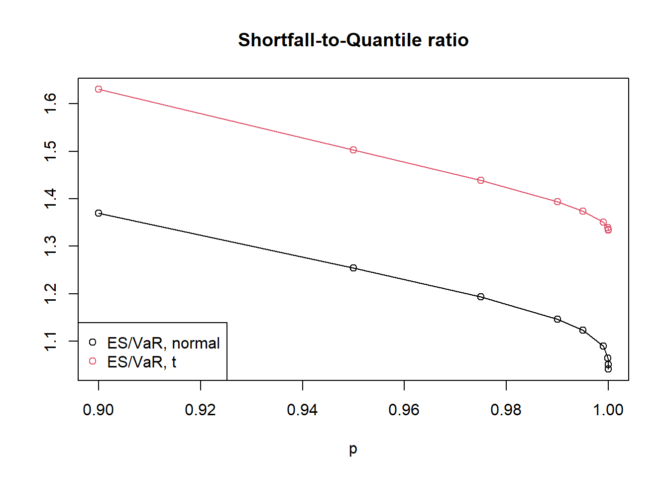
Findings and conclusions
Most risk managers would argue that the t model is riskier than the normal model, since under the t distribution large losses are more likely. However, if we use VaR at the 95% or 97.5% confidence level to measure risk, the normal distribution appears to be at least as risky as the t model; only above a confidence level of 99% does the higher risk in the tails of the t model become apparent.
On the other hand, if we use ES, the risk in the tails of the t model is reflected in our risk measurement for lower values of \(\alpha\). Of course, simply going to a 99% confidence level in quoting VaR numbers does not help to overcome this deficiency of VaR, as there are other examples where the higher risk becomes apparent only for confidence levels beyond 99%.
It is possible to derive results on the asymptotics of the shortfall-to-quantile ratio \(\text{ES}_\alpha/\text{VaR}_\alpha\) for \(\alpha \rightarrow 1\). For the normal distribution we have \(\lim\limits_{\alpha \rightarrow 1} \text{ES}_\alpha/\text{VaR}_\alpha = 1\); for the t distribution with \(\nu > 1\) degrees of freedom we have \(\lim\limits_{\alpha \rightarrow 1} \text{ES}_\alpha/\text{VaR}_\alpha = \nu/(\nu - 1) > 1\). This shows that for a heavy-tailed distribution, the difference between ES and VaR is more pronounced than for the normal distribution.