Basic Terminology
Prerequisite
Install R from https://cran.r-project.org/, as well as an integrated development environment (IDE) (e.g., editor, build tools):
- RStudio: http://www.rstudio.com/.
R (contributed) packages can be installed via either of the following versions.
Release versions:
comprehensive R Archive Network (CRAN): install.packages(“mypkg”);
bioconductor: devtools::install_bioc(“mypackage”) or BiocManager::install(“mypackage”).
Development versions:
R-Forge: install.packages(“mypkg”, repos = “https://R-Forge.R-project.org”));
GitHub: devtools::install_github(“maintainer/mypkg”).
To work with R,
create a script (a file, e.g. myscript.R) containing the R source code; and
run the script interactively by executing it line-by-line.
To run the current line, press Control+R or right-click and select Run line or selection. If you want to understand a command, enter ?command in R console.
This is a good practice: clean all objects from memory before using an R instance.
Creating objects
- Scalars
Run the next line and the value of the object scalar1 appears in the R Console.
## [1] 1- Vectors
## [1] 1 1 1 1 1## [1] 1 2 3 4 5 6 7 8 9 10## [1] 1 4 -7 10 -20## [1] 1 3 5 7 9## [1] 5 5## [1] 1 2 3 4 5 1 2 3 4 5 1 2 3 4 5## [1] 5## [,1] [,2] [,3] [,4] [,5]
## [1,] 1 5 9 13 17
## [2,] 2 6 10 14 18
## [3,] 3 7 11 15 19
## [4,] 4 8 12 16 20## [,1] [,2] [,3] [,4] [,5] [,6]
## [1,] 8 8 8 8 8 8
## [2,] 8 8 8 8 8 8
## [3,] 8 8 8 8 8 8
## [4,] 8 8 8 8 8 8## [1] 4 5## [1] 4 6## [,1] [,2] [,3] [,4] [,5]
## 1 5 9 13 17
## 2 6 10 14 18
## 3 7 11 15 19
## 4 8 12 16 20
## vector1 1 1 1 1 1##
## 10- Strings
## [1] "Hello!"## [1] "Hello!" "Happy New Year."# Combine string1 and string2 with "---" in between
string3 <- paste(string2,collapse="---")
string3## [1] "Hello!---Happy New Year."## NULLlabels <- c("A", "B", "C", "D", "E")
colnames(matrix3) <- paste("Column",labels,sep=" ")
colnames(matrix3)## [1] "Column A" "Column B" "Column C" "Column D" "Column E"## [1] "Row 1" "Row 2" "Row 3" "Row 4" "Row 5"Note: sep is different from collapse.
Basic calculations
- Transpose
##       Column A Column B Column C Column D Column E
## Row 1        1        5        9       13       17
## Row 2        2        6       10       14       18
## Row 3        3        7       11       15       19
## Row 4        4        8       12       16       20
## Row 5 1 1 1 1 1## Row 1 Row 2 Row 3 Row 4 Row 5
## Column A 1 2 3 4 1
## Column B 5 6 7 8 1
## Column C 9 10 11 12 1
## Column D 13 14 15 16 1
## Column E 17 18 19 20 1- Inverse
##        Column A  Column B   Column C   Column D   Column E
## Row 1 1.0000000 0.2000000 0.11111111 0.07692308 0.05882353
## Row 2 0.5000000 0.1666667 0.10000000 0.07142857 0.05555556
## Row 3 0.3333333 0.1428571 0.09090909 0.06666667 0.05263158
## Row 4 0.2500000 0.1250000 0.08333333 0.06250000 0.05000000
## Row 5 1.0000000 1.0000000 1.00000000 1.00000000 1.00000000- Element-by-element multiplication
##       Column A Column B Column C Column D Column E
## Row 1 1.000000 2.236068 3.000000 3.605551 4.123106
## Row 2 1.414214 2.449490 3.162278 3.741657 4.242641
## Row 3 1.732051 2.645751 3.316625 3.872983 4.358899
## Row 4 2.000000 2.828427 3.464102 4.000000 4.472136
## Row 5 1.000000 1.000000 1.000000 1.000000 1.000000## [,1] [,2] [,3] [,4] [,5]
## [1,] 0 5 10 15 20
## [2,] 1 6 11 16 21
## [3,] 2 7 12 17 22
## [4,] 3 8 13 18 23
## [5,] 4 9 14 19 24## Column A Column B Column C Column D Column E
## Row 1 0 25 90 195 340
## Row 2 2 36 110 224 378
## Row 3 6 49 132 255 418
## Row 4 12 64 156 288 460
## Row 5 4 9 14 19 24- Matrix algebra
##       [,1] [,2] [,3] [,4] [,5]
## Row 1  130  355  580  805 1030
## Row 2  140  390  640  890 1140
## Row 3  150  425  700  975 1250
## Row 4  160  460  760 1060 1360
## Row 5   10   35   60   85  110
Consider a matrix from all rows and first three column of matrix4.
##      [,1] [,2] [,3] [,4] [,5]
## [1,] 70 195 320 445 570## [,1] [,2] [,3]
## [1,] 70 195 320Control flow
IfStatement
## [1] "Scalar smaller or equal 4"Forandwhileloops
matrix5 <- matrix(0,nrow(matrix4),ncol(matrix4))
for (i in 1:nrow(matrix4)){
    for (j in 1:ncol(matrix4)){
        matrix5[i,j] <- matrix4[i,j]+i*j
    }
}
matrix5
## [,1] [,2] [,3] [,4] [,5]
## [1,] 1 7 13 19 25
## [2,] 3 10 17 24 31
## [3,] 5 13 21 29 37
## [4,] 7 16 25 34 43
## [5,] 9 19 29 39 49## [,1] [,2] [,3] [,4] [,5]
## [1,] 1 2 3 4 5
## [2,] 2 4 6 8 10
## [3,] 3 6 9 12 15
## [4,] 4 8 12 16 20
## [5,] 5 10 15 20 25This is the while-loop equivalent to the for-loop above:
matrix6 <- matrix(0,nrow(matrix4),ncol(matrix4))
i <- 1
while (i<=nrow(matrix4)){
    j <- 1
    while (j<=nrow(matrix4)){
        matrix6[i,j] <- matrix4[i,j]+i*j
        j <- j+1
    }
    i <- i+1
}
matrix5-matrix6
## [,1] [,2] [,3] [,4] [,5]
## [1,] 0 0 0 0 0
## [2,] 0 0 0 0 0
## [3,] 0 0 0 0 0
## [4,] 0 0 0 0 0
## [5,] 0 0 0 0 0Random number generation
- Generate random numbers from a normal distribution.
## [1] -0.520841792 -0.005744297 0.952890749 0.715788002 -0.521479412## [1] 3.958241 1.419152 6.538898 5.120411 7.084203## [1] 0.05844094## [1] 0.0249979## [1] -1.96- Generate random numbers from a student-t distribution.
## [1] 1.3244122 0.3202999 0.1944042 2.4318852 0.3439128## [1] 4.427300 9.591149 14.683066 10.542664 12.879060## [1] 0.06968985## [1] 0.06077732## [1] -2.131847- Generate pseudo random numbers with/out replacement.
## [1] 9 7 8 5 10 2 4 1 3 6## [1] 9 7 10 1 6 6 8 5 9 8- Control the draws (this is pseudo-random afterall).
The set.seed() function in R is used to create reproducible results when writing code that involves creating variables that take on random values. By using the set.seed() function, you guarantee that the same random values are produced each time you run the code.
## [1] -0.84085548 1.38435934 -1.25549186 0.07014277 1.71144087# By calling the seed you stored, you can retrive the 5 numbers just generated.
set.seed(your.choice)
rnorm(5)## [1] -0.84085548 1.38435934 -1.25549186 0.07014277 1.71144087## [1] -0.6029080 -0.4721664 -0.6353713 -0.2857736 0.1381082Data and dates
R provides some data sets. For example, see available data sets.
## Grouped Data: circumference ~ age | Tree
##    Tree  age circumference
## 1     1  118            30
## 2     1  484            58
## 3     1  664            87
## 4     1 1004           115
## 5     1 1231           120
## 6     1 1372           142
## 7     1 1582           145
## 8     2  118            33
## 9     2  484            69
## 10    2  664           111
## 11    2 1004           156
## 12    2 1231           172
## 13    2 1372           203
## 14    2 1582           203
## 15    3  118            30
## 16    3  484            51
## 17    3  664            75
## 18    3 1004           108
## 19    3 1231           115
## 20    3 1372           139
## 21    3 1582           140
## 22    4  118            32
## 23    4  484            62
## 24    4  664           112
## 25    4 1004           167
## 26    4 1231           179
## 27    4 1372           209
## 28    4 1582           214
## 29    5  118            30
## 30    5  484            49
## 31    5  664            81
## 32    5 1004           125
## 33    5 1231           142
## 34    5 1372           174
## 35    5 1582           177
See available objects in this R instance’s memory (ls=list of objects).
##  [1] "dof"                "i"                  "j"                  "labels"             "matrix1"
##  [6] "matrix2"            "matrix3"            "matrix4"            "matrix5"            "matrix6"
## [11] "rand.norm"          "repeated.sequence1" "repeated1"          "scalar1"            "sequence1"
## [16] "sequence2"          "sequence3"          "string1"            "string2"            "string3"
## [21] "vector1"            "your.choice"
Convert part of Orange to time series.
## Time Series:
## Start = 1995
## End = 2000
## Frequency = 1
##      Tree  age circumference
## 1995    1  118            30
## 1996    1  484            58
## 1997    1  664            87
## 1998    1 1004           115
## 1999    1 1231           120
## 2000    1 1372           142
Some basic ts commands.
## [1] 1995 1## [1] 2000 1## Time Series:
## Start = 1996
## End = 2000
## Frequency = 1
## [1] 28 29 28 5 22## Time Series:
## Start = 1993
## End = 1998
## Frequency = 1
## [1] 30 58 87 115 120 142## Time Series:
## Start = 1993
## End = 2000
## Frequency = 1
## Orange1TS.Tree Orange1TS.age Orange1TS.circumference diff(Orange1TS[, 3]) lag(Orange1TS[, 3], 2)
## 1993 NA NA NA NA 30
## 1994 NA NA NA NA 58
## 1995 1 118 30 NA 87
## 1996 1 484 58 28 115
## 1997 1 664 87 29 120
## 1998 1 1004 115 28 142
## 1999 1 1231 120 5 NA
## 2000 1 1372 142 22 NAWriting functions
R makes writing user-defined function very easy. This makes sense whenever you have to repeat a specific sequence of commands on similar objects. Commenting is very useful to remind you of what a function 1) needs as input, 2) does and 3) gives out.
summarize.matrix <- function(mat){
    # Plots columns of a matrix into one graph and returns summary statistics
    nc <- ncol(mat)
    dev.new()
    plot(mat[,1], type="l", ylim=c(min(mat),max(mat)))
      # Plot the first column of mat using line. Set the y axis between maximum and minimum values
    if (nc>1) for (j in 2:nc) lines(mat[,j],col=j)
    legend("bottomleft",paste("Column",1:nc,sep=" "), col=1:nc, lty=1, cex=.8)
    return(summary(mat))
}

summarize.matrix(matrix1)
## V1 V2 V3 V4 V5
## Min. :1.00 Min. :5.00 Min. : 9.00 Min. :13.00 Min. :17.00
## 1st Qu.:1.75 1st Qu.:5.75 1st Qu.: 9.75 1st Qu.:13.75 1st Qu.:17.75
## Median :2.50 Median :6.50 Median :10.50 Median :14.50 Median :18.50
## Mean :2.50 Mean :6.50 Mean :10.50 Mean :14.50 Mean :18.50
## 3rd Qu.:3.25 3rd Qu.:7.25 3rd Qu.:11.25 3rd Qu.:15.25 3rd Qu.:19.25
## Max. :4.00 Max. :8.00 Max. :12.00 Max. :16.00 Max. :20.00## V1 V2 V3 V4 V5 V6
## Min. :8 Min. :8 Min. :8 Min. :8 Min. :8 Min. :8
## 1st Qu.:8 1st Qu.:8 1st Qu.:8 1st Qu.:8 1st Qu.:8 1st Qu.:8
## Median :8 Median :8 Median :8 Median :8 Median :8 Median :8
## Mean :8 Mean :8 Mean :8 Mean :8 Mean :8 Mean :8
## 3rd Qu.:8 3rd Qu.:8 3rd Qu.:8 3rd Qu.:8 3rd Qu.:8 3rd Qu.:8
## Max. :8 Max. :8 Max. :8 Max. :8 Max. :8 Max. :8## Column A Column B Column C Column D Column E
## Min. :1.0 Min. :1.0 Min. : 1.0 Min. : 1.0 Min. : 1
## 1st Qu.:1.0 1st Qu.:5.0 1st Qu.: 9.0 1st Qu.:13.0 1st Qu.:17
## Median :2.0 Median :6.0 Median :10.0 Median :14.0 Median :18
## Mean :2.2 Mean :5.4 Mean : 8.6 Mean :11.8 Mean :15
## 3rd Qu.:3.0 3rd Qu.:7.0 3rd Qu.:11.0 3rd Qu.:15.0 3rd Qu.:19
## Max. :4.0 Max. :8.0 Max. :12.0 Max. :16.0 Max. :20## V1 V2 V3 V4 V5
## Min. :0 Min. :5 Min. :10 Min. :15 Min. :20
## 1st Qu.:1 1st Qu.:6 1st Qu.:11 1st Qu.:16 1st Qu.:21
## Median :2 Median :7 Median :12 Median :17 Median :22
## Mean :2 Mean :7 Mean :12 Mean :17 Mean :22
## 3rd Qu.:3 3rd Qu.:8 3rd Qu.:13 3rd Qu.:18 3rd Qu.:23
## Max. :4 Max. :9 Max. :14 Max. :19 Max. :24## V1 V2 V3 V4 V5
## Min. :1 Min. : 7 Min. :13 Min. :19 Min. :25
## 1st Qu.:3 1st Qu.:10 1st Qu.:17 1st Qu.:24 1st Qu.:31
## Median :5 Median :13 Median :21 Median :29 Median :37
## Mean :5 Mean :13 Mean :21 Mean :29 Mean :37
## 3rd Qu.:7 3rd Qu.:16 3rd Qu.:25 3rd Qu.:34 3rd Qu.:43
## Max. :9 Max. :19 Max. :29 Max. :39 Max. :49For example, concerning “data(Orange)”,
##       Tree        age         circumference
##  Min.   :1   Min.   : 118.0   Min.   : 30.00
##  1st Qu.:1   1st Qu.: 529.0   1st Qu.: 65.25
##  Median :1   Median : 834.0   Median :101.00
##  Mean   :1   Mean   : 812.2   Mean   : 92.00
##  3rd Qu.:1   3rd Qu.:1174.2   3rd Qu.:118.75
##  Max.   :1   Max.   :1372.0   Max.   :142.00
More
Much has been programmed before and is provided for free in packages. You need to install them, but the common ones are already available on LSE computers. Load them using library("packagename"):
See the code of a self-defined function or a function from a package by typing in its name:
## function (mat)
## {
##     nc <- ncol(mat)
##     dev.new()
##     plot(mat[, 1], type = "l", ylim = c(min(mat), max(mat)))
##     if (nc > 1)
##         for (j in 2:nc) lines(mat[, j], col = j)
##     legend("bottomleft", paste("Column", 1:nc, sep = " "), col = 1:nc,
##         lty = 1, cex = 0.8)
##     return(summary(mat))
## }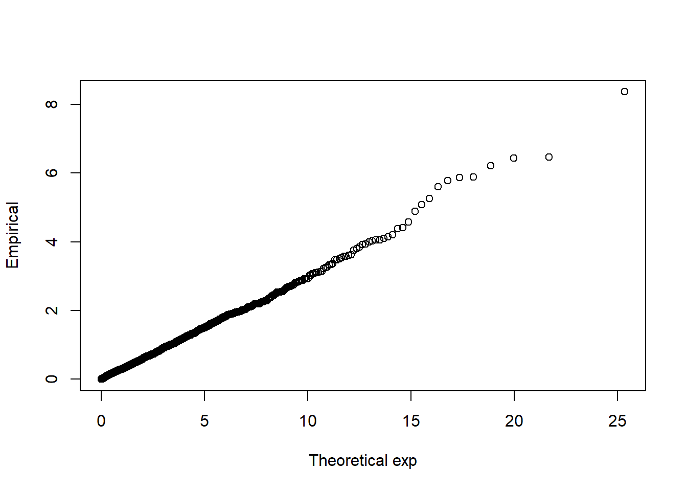
## <environment: 0x000001436f8c93b0>## function (x, a = 0.5, reference = c("normal", "exp", "student"),
## ...)
## {
## n <- length(x)
## reference <- match.arg(reference)
## plot.points <- ppoints(n, a)
## func <- switch(reference, normal = qnorm, exp = qexp, student = qt)
## xp <- func(plot.points, ...)
## y <- sort(x)
## plot(xp, y, xlab = paste("Theoretical", reference), ylab = "Empirical")
## invisible(list(x = x, y = y))
## }
## <bytecode: 0x000001436f6f37e0>
## <environment: namespace:QRM>For more information, references and examples add a ‘?’, e.g. ‘?QQplot’.
You can find much reading material online for free. Some good reads can be:
A R introduction: http://cran.r-project.org/doc/manuals/R-intro.pdf
On good coding style: short - http://adv-r.had.co.nz/Style.html
… detailed: http://cran.r-project.org/web/packages/rockchalk/vignettes/Rstyle.pdf