Portfolio Risk Measures - PART II
Case study
The goal of this mini project is to use the techniques of Normality Test and Principal Component Analysis we learned in the lecture to analyse Dow Jones 30 stock prices daily from 1991-01-02 to 2000-12-29. The dataset is provided by loading the libraries of QRM and qrmtools, which offer comprehensive functions for modelling and managing risk.
To complete the tasks of this session, you should also require the following libraries.
To access the data, alongside a list of constituent names, we conduct the following code:
## [1] "AA" "AXP" "T" "BA" "CAT" "C" "KO" "DD" "EK" "XOM" "GE" "GM" "HWP" "HD" "HON"
## [16] "INTC" "IBM" "IP" "JPM" "JNJ" "MCD" "MRK" "MSFT" "MMM" "MO" "PG" "SBC" "UTX" "WMT" "DIS"You select 10 out of 30 companies from the list above to form your own portfolio.
The list below outlines the tasks that you need to complete.
Normality Tests:
Construct daily, weekly, monthly and quarterly returns of your selected stocks for the period 01/01/1993-31/12/2000.
Conduct Mardia’s tests of multivariate normality on the daily, weekly, monthly and annual returns, with the confidence level suggested to be 95%.
Conduct Jarque-Bera test of univariate normality on each column in the dataset of the periodic returns.
Principal Component Analysis:
Use the Dow Jones Index as the benchmark returns, i.e., \(\mu\), which can be accessed by
data(dji). Construct and calculate the daily log-returns of the index corresponding to the same observation window.Apply the spectral decomposition to find the eigenvalues and eigenvectors of your selected stocks.
Calculate the principal components, compute the cumulative contribution to the total variance, and plot your results.
Reference codes
Ensure you clean your current workspace before running any R scripts for optimal performance.
- Load libraries and data.
library("QRM")
library("qrmtools")
library("mvtnorm")
library("xts")
library("tseries")
library("factoextra") # Package for PCA visualization## [1] "AA" "AXP" "T" "BA" "CAT" "C" "KO" "DD" "EK" "XOM" "GE" "GM" "HWP" "HD" "HON"
## [16] "INTC" "IBM" "IP" "JPM" "JNJ" "MCD" "MRK" "MSFT" "MMM" "MO" "PG" "SBC" "UTX" "WMT" "DIS"Normality Tests.
- Select 10 out of 30 companies and construct a time series of their stock prices.
stock.selection <- c("MO","KO","EK","HWP","INTC","MSFT","IBM","MCD","WMT","DIS")
prices <- DJ[,stock.selection]
head(prices, 3)
## GMT
## MO KO EK HWP INTC MSFT IBM MCD WMT DIS
## 1991-01-02 10.5506 9.8760 23.0207 3.9108 1.1968 2.0764 27.8566 7.0782 7.0547 7.8604
## 1991-01-03 10.2654 9.6032 22.9507 3.9108 1.1968 2.0903 27.9498 6.9851 7.0547 7.8215
## 1991-01-04 10.2395 9.8487 22.7408 3.8492 1.2046 2.1076 27.8566 7.0161 6.9665 7.7923- Calculate the log-prices/returns of your selected stocks.
## GMT
##                  MO       KO       EK      HWP      INTC      MSFT     IBM      MCD      WMT      DIS
## 1991-01-02 2.356183 2.290108 3.136394 1.363742 0.1796513 0.7306356 3.32707 1.957020 1.953694 2.061837
## 1991-01-03 2.328779 2.262096 3.133348 1.363742 0.1796513 0.7373076 3.33041 1.943779 1.953694 2.056876
## 1991-01-04 2.326253 2.287339 3.124161 1.347865 0.1861476 0.7455499 3.32707 1.948208 1.941113 2.053136## GMT
## MO KO EK HWP INTC MSFT IBM MCD
## 1991-01-02 NA NA NA NA NA NA NA NA
## 1991-01-03 -0.027403713 -0.02801120 -0.003045374 0.00000000 0.000000000 0.006671971 0.003340122 -0.013240329
## 1991-01-04 -0.002526227 0.02524309 -0.009187769 -0.01587662 0.006496233 0.008242263 -0.003340122 0.004428199
## WMT DIS
## 1991-01-02 NA NA
## 1991-01-03 0.00000000 -0.004961144
## 1991-01-04 -0.01258111 -0.003740285- Generate daily, weekly, monthly and quarterly returns for the period 01/01/1993-31/12/2000.
# Set up the observation window.
start.date <- timeCalendar(d=1,m=1,y=1993)
end.date <- timeCalendar(d=31,m=12,y=2000)## GMT
## MO KO EK HWP INTC MSFT IBM MCD
## 1993-01-04 -0.009770992 0.002980470 0.00921909 -0.02536816 -0.005784864 -0.002927875 -0.00497376 0.005115859
## 1993-01-05 -0.038368795 -0.021052283 0.02417146 0.02715578 0.050720405 0.016016750 -0.02525502 -0.005115859
## 1993-01-06 -0.022357554 0.006060298 0.01481383 0.03852908 0.080455953 0.028501204 -0.01806417 0.005115859
## WMT DIS
## 1993-01-04 -0.017731728 -0.005834979
## 1993-01-05 -0.003981952 0.007052471
## 1993-01-06 -0.026290350 0.022984826# Generate the weekly returns.
by <- timeSequence(from = start.date, to = end.date, by = "week")
X.weekly <- aggregate(X.daily, by, sum)
head(X.weekly, 3)## GMT
## MO KO EK HWP INTC MSFT IBM MCD
## 1993-01-08 -0.041360853 -0.03958237 0.03039892 0.012446760 0.126662785 0.020295283 -0.08004138 0.01526972
## 1993-01-15 -0.017034284 0.07188892 0.14728506 0.029586987 0.123669259 0.029690911 0.03694181 0.00000000
## 1993-01-22 -0.006895799 -0.05342234 0.01028333 0.006838848 -0.002247904 -0.004198196 0.00774399 -0.02298876
## WMT DIS
## 1993-01-08 -0.07500427 0.004118734
## 1993-01-15 0.01876717 0.039778811
## 1993-01-22 0.03452342 -0.014025256# Generate the monthly returns.
by <- timeSequence(from = start.date, to = end.date, by = "month")
X.monthly <- aggregate(X.daily, by, sum)
head(X.monthly, 3)## GMT
## MO KO EK HWP INTC MSFT IBM MCD
## 1993-02-01 -0.016338434 0.02650974 0.20319343 0.043747849 0.24586009 0.02460165 0.04369213 0.010205679
## 1993-03-01 -0.150860571 -0.02055765 0.06607521 0.003419414 0.03531165 -0.07103510 0.03960127 0.007582427
## 1993-04-01 -0.007403213 0.02153990 0.03738810 0.031914237 -0.03308760 0.13198666 -0.05394390 0.075186498
## WMT DIS
## 1993-02-01 0.028880128 0.06047087
## 1993-03-01 0.001894728 -0.04196360
## 1993-04-01 -0.057542567 0.01699591# Generate the quarterly returns.
by <- timeSequence(from = start.date, to = end.date, by = "quarter")
X.quarterly <- aggregate(X.daily,by,sum)
head(X.quarterly, 3)## GMT
## MO KO EK HWP INTC MSFT IBM MCD
## 1993-04-01 -0.17460222 0.027491988 0.30665674 0.07908150 0.2480841 0.08555320 0.0293495 0.09297460
## 1993-07-01 -0.26863069 0.007105448 -0.06918209 0.05310853 -0.0318939 -0.06525792 -0.0519166 -0.08785874
## 1993-10-01 -0.03677305 -0.019579060 0.17247651 -0.14659544 0.3014893 -0.06062233 -0.1155608 0.06899506
## WMT DIS
## 1993-04-01 -0.02676771 0.03550317
## 1993-07-01 -0.18837533 -0.08661695
## 1993-10-01 -0.03836991 -0.07163943Conduct Mardia’s test of multivariate normality on each set of the periodic returns.
Recall that Mardia’s test of multivariate normality relies on a hypothesis test on the multivariate measures of skewness (
K3) and kurtosis (K4) with their corresponding asymptotic distributions:\[ \frac{n}{6} K_3 \sim \chi^2_{d(d+1)(d+2)/6}, \qquad \frac{K_4-d(d+2)}{\sqrt{8d(d+2)/n}} \sim \mathcal{N}(0,1). \]
Consider rejecting the null hypothesis that the periodic returns of the selected stocks follow some multivariate normal distribution in the event that the resulting p-value < 0.05.
##         K3 K3 p-value         K4 K4 p-value
## 10.86037 0.00000 263.76064 0.00000## K3 K3 p-value K4 K4 p-value
## 11.90346 0.00000 187.48002 0.00000## K3 K3 p-value K4 K4 p-value
## 2.484269e+01 6.166512e-12 1.471844e+02 0.000000e+00## K3 K3 p-value K4 K4 p-value
## 46.1454125 0.1877432 117.3633980 0.3178233Conduct Jarque-Bera test of univariate normality on each column in the periodic returns, with the test stats given by:
\[ T = \frac{n}{6}\left( K_3^2 + \frac{(K_4-3)^2}{4} \right) \sim \chi^2_2. \] When \(T\) value is far from 0, it may lead to the rejection of normality.
As this test is univariate, we run it for each column in a dataset separately.
# To repeat as little as possible, we write a short function for this.
JBTest <- function(dataMatrix){
    ncol <- dim(dataMatrix)[2]
    pvals <- array(NA, ncol)
    for (i in 1:ncol) pvals[i] <- jarque.bera.test(dataMatrix[,i])$p.value
    if (!is.null(names(dataMatrix))) names(pvals) <- names(dataMatrix)
    return(pvals)
}## MO KO EK HWP INTC MSFT IBM MCD WMT DIS
## 0 0 0 0 0 0 0 0 0 0## MO KO EK HWP INTC MSFT IBM MCD
## 0.000000e+00 1.627990e-08 0.000000e+00 3.734235e-12 0.000000e+00 0.000000e+00 2.114411e-04 3.195393e-03
## WMT DIS
## 1.968471e-03 1.037249e-08## MO KO EK HWP INTC MSFT IBM MCD
## 1.397525e-09 5.602451e-02 0.000000e+00 2.800529e-01 3.330669e-16 6.864336e-02 7.929228e-01 6.819415e-01
## WMT DIS
## 9.926543e-01 8.899040e-01## MO KO EK HWP INTC MSFT IBM MCD
## 0.1074131679 0.0004216985 0.0919092699 0.9000812140 0.5390802680 0.5933648016 0.2917917380 0.6176245067
## WMT DIS
## 0.3374939877 0.0534219356Principal Component Analysis.
To the selected 10 stocks, they have been chosen to be of two types:
- technology-related titles like Hewlett-Packard, Intel, Microsoft and IBM; and
- food/consumer-related titles like Philip Morris, Coca-Cola, Eastman Kodak, McDonald’s, Wal-Mart and Disney.
- Prepare data for the benchmark means \(\mu\), the daily log-returns of the Dow Jones Index.
# Load the index level data.
data(dji)
# Calculate the index returns corresponding to the same window.
X.ind <- diff(log(dji))
X.ind <- window(X.ind,start.date,end.date)
Consider returns relative to the benchmark: subtract them from the stock returns.
# We repeat the index returns for each selected stocks.
X <- X.daily - X.ind[,rep(1,ncol(X.daily))]
head(X, 3)
## GMT
## MO KO EK HWP INTC MSFT IBM
## 1993-01-04 -0.01222473 0.0005267335 0.006765354 -0.02782189 -0.008238601 -0.005381612 -0.007427496
## 1993-01-05 -0.03796076 -0.0206442482 0.024579490 0.02756381 0.051128440 0.016424785 -0.024846983
## 1993-01-06 -0.02153796 0.0068798919 0.015633421 0.03934867 0.081275547 0.029320798 -0.017244577
## MCD WMT DIS
## 1993-01-04 0.002662123 -0.020185464 -0.008288715
## 1993-01-05 -0.004707825 -0.003573918 0.007460505
## 1993-01-06 0.005935453 -0.025470756 0.023804420- Apply spectral decomposition.
# Note: R computes the unbiased sample covariance.
S <- var(X)
# Get the eigenvalues/vectors.
tmp.eigen <- eigen(S)
names(tmp.eigen)
## [1] "values" "vectors"L <- diag(tmp.eigen$values) # eigenvalues
G <- tmp.eigen$vectors # eigenvectors
# Check spectral decomposition (first 3 by 3 minor)
check <- G %*% L %*% t(G)
max(abs(S-check)) # the maximum discrepancy due to the rounding errors## [1] 4.336809e-19Calculate principal components.
Now, all the resources are available to conduct the PCA analysis. First, the
princomp()computes the PCA, andsummary()function shows the result.
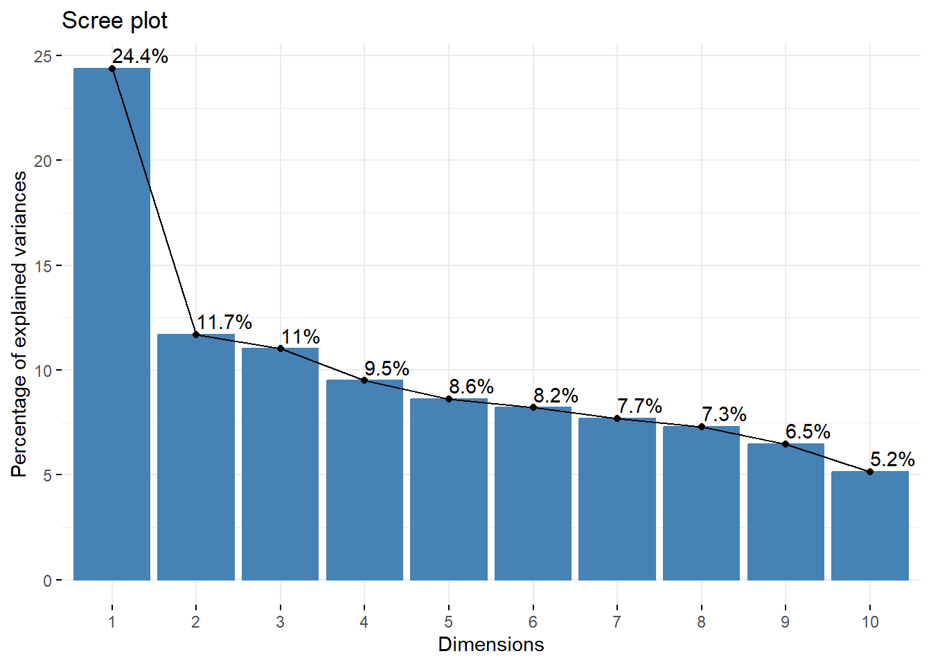
## Importance of components:
##                            Comp.1    Comp.2     Comp.3     Comp.4     Comp.5     Comp.6     Comp.7     Comp.8
## Standard deviation     0.03094445 0.0214188 0.02078997 0.01930529 0.01840345 0.01794285 0.01737690 0.01692016
## Proportion of Variance 0.24388101 0.1168431 0.11008301 0.09492164 0.08626035 0.08199651 0.07690541 0.07291574
## Cumulative Proportion  0.24388101 0.3607241 0.47080707 0.56572871 0.65198906 0.73398557 0.81089098 0.88380672
##                            Comp.9    Comp.10
## Standard deviation     0.01593690 0.01422073
## Proportion of Variance 0.06468744 0.05150585
## Cumulative Proportion 0.94849415 1.00000000##
## Loadings:
## Comp.1 Comp.2 Comp.3 Comp.4 Comp.5 Comp.6 Comp.7 Comp.8 Comp.9 Comp.10
## MO 0.192 0.916 0.249 0.156 0.146
## KO 0.106 0.213 0.113 -0.122 -0.574 -0.758
## EK 0.183 -0.186 -0.804 0.277 0.418 -0.148 -0.106
## HWP -0.518 0.739 -0.122 0.258 -0.156 0.161 -0.215
## INTC -0.672 -0.445 0.138 0.563
## MSFT -0.431 -0.336 0.150 0.189 -0.186 -0.765 -0.143
## IBM -0.270 0.262 -0.376 0.424 -0.123 0.646 -0.175 -0.231 -0.119
## MCD 0.187 0.110 0.170 -0.711 0.638
## WMT -0.169 -0.191 0.688 0.150 0.355 0.510 0.226
## DIS 0.152 0.392 -0.241 -0.839 0.219
##
## Comp.1 Comp.2 Comp.3 Comp.4 Comp.5 Comp.6 Comp.7 Comp.8 Comp.9 Comp.10
## SS loadings 1.0 1.0 1.0 1.0 1.0 1.0 1.0 1.0 1.0 1.0
## Proportion Var 0.1 0.1 0.1 0.1 0.1 0.1 0.1 0.1 0.1 0.1
## Cumulative Var 0.1 0.2 0.3 0.4 0.5 0.6 0.7 0.8 0.9 1.0Next we should check that the sum of variances of PCs equals the sum of variances of the original data.
## [1] 0.003926336## [1] 0.003928281# Cumulative contribution to the total variance
ratio <- cumsum(PC.variances)/sum(PC.variances)
ratio## Comp.1 Comp.2 Comp.3 Comp.4 Comp.5 Comp.6 Comp.7 Comp.8 Comp.9 Comp.10
## 0.2438810 0.3607241 0.4708071 0.5657287 0.6519891 0.7339856 0.8108910 0.8838067 0.9484942 1.0000000Visualization of the principal components.
To visualize the importance of each principal component and to determine the number of principal components to retain, the scree plot is employed by using the
fviz_eig()function. This plot shows the eigenvalues in a downward curve, from highest to lowest.To visualize the similarities and dissimilarities between the samples, and to show the impact of each attribute on each of the principal components, we can use the
fviz_pca_varfunction.
## Warning in geom_bar(stat = "identity", fill = barfill, color = barcolor, : Ignoring empty aesthetic: `width`.
fviz_pca_var(out,
             col.var = "contrib", # Color by contributions to the PC
             gradient.cols = c("#00AFBB", "#E7B800", "#FC4E07"),
             repel = TRUE     # Avoid text overlapping
             )
## Warning: Using `size` aesthetic for lines was deprecated in ggplot2 3.4.0.
## ℹ Please use `linewidth` instead.
## ℹ The deprecated feature was likely used in the ggpubr package.
## Please report the issue at <https://github.com/kassambara/ggpubr/issues>.
## This warning is displayed once every 8 hours.
## Call `lifecycle::last_lifecycle_warnings()` to see where this warning was generated.