Portfolio Risk Measures - PART I

Case study

The goal of this mini project is to use the techniques we learned in the lecture to analyse Dow Jones 30 stock prices daily from 1991-01-02 to 2000-12-29. The dataset is provided by loading the libraries of QRM and qrmtools, which offer comprehensive functions for modelling and managing risk.

library("QRM")
library("qrmtools")

To access the data, alongside a list of constituent names, we conduct the following code:

data(DJ)        # Dow Jones 30 stock prices
names(DJ)       # List constituents

##  [1] "AA"   "AXP"  "T"    "BA"   "CAT"  "C"    "KO"   "DD"   "EK"   "XOM"  "GE"   "GM"   "HWP"  "HD"   "HON"  "INTC"
## [17] "IBM"  "IP"   "JPM"  "JNJ"  "MCD"  "MRK"  "MSFT" "MMM"  "MO"   "PG"   "SBC"  "UTX"  "WMT"  "DIS"

You select d out of 30 companies from the list above to form your own portfolio, with an arbitrary number of shares assigned to each company in the portfolio. For instance, if I choose the 4 companies: “General Electric”, “Intel”, “Coca Cola” and “Johnson & Johnson”, each with an equal number of shares, I would define it in the code as follows:

stock.selection <- c("GE","INTC","KO","JNJ") 
# with number of shares of each company in the portfolio
lambda <- c(1000,1000,1000,1000)

The list below outlines the analysis that you need to perform, with the confidence level for your risk measures suggested to be 99%.

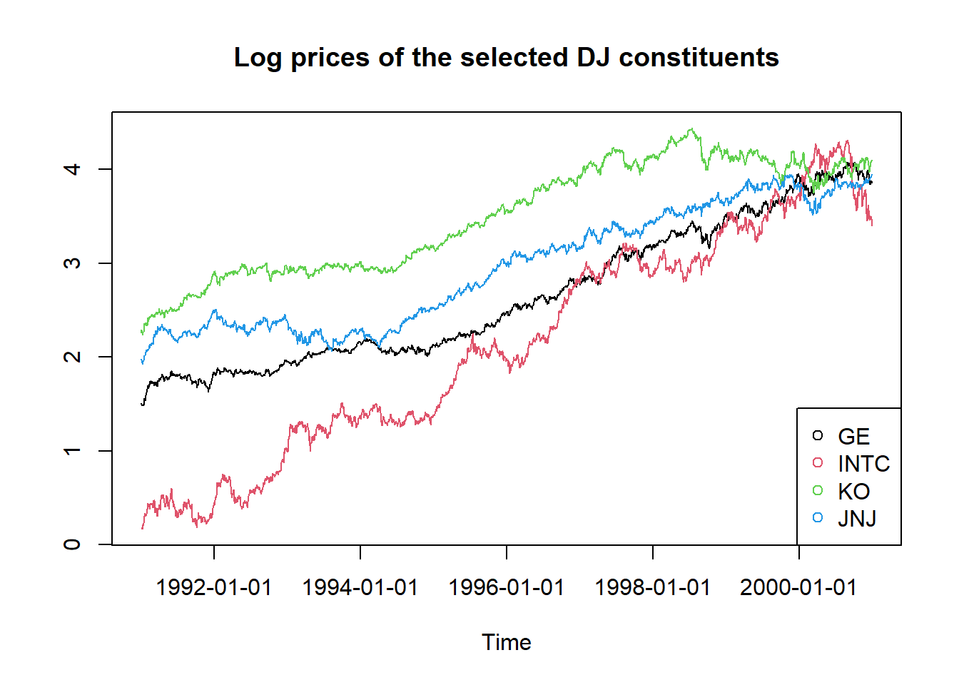
Prepare the data set for your portfolio so that it can be analysed by R.
Construct and plot the time series of the log prices of your selected stocks.
Plot the scatter plots for the log return pairs among your selected stocks, with a reference to the built-in function pairs().
Construct a loss operator function and find
- the losses of selected stocks over the full sample period;
- the losses of selected stocks on the first day; and
- the linearised losses of selected stocks on the first day.
Construct unbiased estimates for the mean and covariance for the stocks in your portfolio.
Calculate the value-at-risk and expected shortfall for your portfolio losses
- with an assumption of normal distribution; and
- without making any assumptions about the underlying distribution.

Reference codes

Load libraries and data.

library("QRM")
library("qrmtools")

data(DJ)     # Dow Jones 30 stock prices
names(DJ)    # List constituents

##  [1] "AA"   "AXP"  "T"    "BA"   "CAT"  "C"    "KO"   "DD"   "EK"   "XOM"  "GE"   "GM"   "HWP"  "HD"   "HON"  "INTC"
## [17] "IBM"  "IP"   "JPM"  "JNJ"  "MCD"  "MRK"  "MSFT" "MMM"  "MO"   "PG"   "SBC"  "UTX"  "WMT"  "DIS"

For the companies above, please see http://money.cnn.com/data/dow30/ for details.

Set parameters.

Choose the following companies and allocate 1000 shares to each: General Electric, Intel, Coca Cola, and Johnson & Johnson. Further set the confidence level \(\alpha\) to 99%.

stock.selection <- c("GE","INTC","KO","JNJ")
# Number of shares of each company in the portfolio
lambda <- c(1000,1000,1000,1000)
# Quantile probability
alpha <- 0.99

Select, transform and plot data.

# Refine the dataset with selected stocks.
prices <- DJ[,stock.selection]

Note: returns are defined as value changes, therefore we will always have one observation less of returns than prices. To be able to put both next to another, we discard the first price observation after computing the return series. Thus, we define \[ r(t) = \log\frac{P(t)}{P(t-1)}, \quad t = 1,2, \dots \] and then we delete \(P(1)\).

# Calcualte the log prices and returns for the selected stocks.
logprices <- log(prices)
logreturns <- diff(logprices)[2:nrow(logprices),]
T <- nrow(logreturns)

prices <- prices[2:(T+1),]
head(prices, 5)

## GMT
##                GE   INTC     KO    JNJ
## 1991-01-03 4.5259 1.1968 9.6032 7.2298
## 1991-01-04 4.4747 1.2046 9.8487 7.1776
## 1991-01-07 4.4031 1.1929 9.6850 6.9558
## 1991-01-08 4.4440 1.1813 9.6032 7.0210
## 1991-01-09 4.4338 1.1929 9.3849 6.8514

logprices <- logprices[2:(T+1),]
head(logprices, 5)

## GMT
##                  GE      INTC       KO      JNJ
## 1991-01-03 1.509816 0.1796513 2.262096 1.978211
## 1991-01-04 1.498439 0.1861476 2.287339 1.970965
## 1991-01-07 1.482309 0.1763873 2.270578 1.939576
## 1991-01-08 1.491555 0.1666155 2.262096 1.948906
## 1991-01-09 1.489257 0.1763873 2.239102 1.924453

# Plot time series of log prices.
plot(logprices[,1],type="l",ylim=c(min(logprices),max(logprices)),ylab="")
title("Log prices of the selected DJ constituents")
lines(logprices[,2],type="l",col=2)
lines(logprices[,3],type="l",col=3)
lines(logprices[,4],type="l",col=4)
legend("bottomright", legend = stock.selection, col=1:4, pch=1)

# Plot scatter plots of return pairs.
pairs(logreturns)

Generate the portfolio.

# Portfolio values
pf.value <- sum(lambda*prices[T,])
pf.value

## [1] 189882.3

# Portfolio weights
pf.weights <- lambda*prices[T,]/pf.value
pf.weights

## GMT
##                   GE      INTC        KO       JNJ
## 2000-12-29 0.2496099 0.1580353 0.3185157 0.2738391

Construct a loss operator function.

Recall that there are three inputs required for defining a loss function lo.fn: log returns x, as the risk factors, the portfolio weights weights and the portfolio value value.

lo.fn <- function(x, weights, value, linear=FALSE){
  # parameter x should be a matrix or vector of N returns (risk-factors)
  # parameter lo.weights should be a vector of N weights
  # parameter lo.value should be a scalar representing a portfolio value
  # On the parameter 'linear': the default is nonlinear which means the
  # function which calculated the return factor (e.g. mk.returns() used
  # a default log() (or some other nonlinear) transform.  Hence using
  # exp(x) will reconvert the log() so the summand will reflect actual
  # changes in value
  
    if ((!(is.vector(x))) & (!(is.matrix(x))))
            stop("x must be vector or matrix with rows corresponding to risk
        factor return observations")
    N <- length(weights)
    T <- 1
    if (is.matrix(x)) T <- dim(x)[1]
    # Weights in a matrix
    weight.mat <- matrix(weights,nrow=T,ncol=N,byrow=TRUE)
    # Starting values for each individual risk factor in matrix form
    tmp.mat <- value * weight.mat

  if (linear) { summand <- x*tmp.mat } else { summand <- (exp(x)-1)*tmp.mat }

  # We return a vector where each row is the change in value summed across
  # each of the risk factors on a single day.
  # By taking the negative we convert to losses
    loss <- -rowSums(summand)
    return(loss)
}

Applying this function to find the (linearised) loss of the selected stocks over full sample period and on the first day.

# Losses of selected stocks over full sample period
loss <- lo.fn(logreturns,pf.weights,pf.value)
# Losses of selected stocks on the first day
lo.fn(logreturns[1,],pf.weights,pf.value)

## 1991-01-03 
##   3276.365

# Losses of selected stocks on the first day, linearized
lo.fn(logreturns[1,],pf.weights,pf.value,linear=TRUE)

## 1991-01-03 
##   3314.653

Variance-covariance analysis.

# Mean and variance adjusted for the R-implied Bessel correction
mu.hat <- colMeans(logreturns)
mu.hat

##           GE         INTC           KO          JNJ 
## 0.0009209655 0.0012754616 0.0007174242 0.0007768039

Make sure you multiply (T-1)/T to get an unbiased estimator for the covariance matrix.

sigma.hat <- var(logreturns)*(T-1)/T
sigma.hat

##                GE         INTC           KO          JNJ
## GE   2.328855e-04 1.155338e-04 9.674371e-05 8.784315e-05
## INTC 1.155338e-04 7.378999e-04 5.180727e-05 7.035340e-05
## KO   9.674371e-05 5.180727e-05 2.857686e-04 9.671003e-05
## JNJ  8.784315e-05 7.035340e-05 9.671003e-05 2.688043e-04

# Find the mean of the portfolio loss.
meanloss <- -sum(pf.weights*mu.hat)*pf.value
meanloss

## [1] -165.7065

# Find the variance of the portfolio loss.
varloss <- pf.value^2 *(pf.weights %*% sigma.hat %*% t(pf.weights))
varloss

##         [,1]
## [1,] 5291842

# Find the VaR of the portfolio loss.
VaR.normal <- meanloss + sqrt(varloss) * qnorm(alpha)
VaR.normal

##          [,1]
## [1,] 5185.825

# Find the ES of the portfolio loss.
ES.normal <- meanloss + sqrt(varloss) * dnorm(qnorm(alpha))/(1-alpha)
ES.normal

##          [,1]
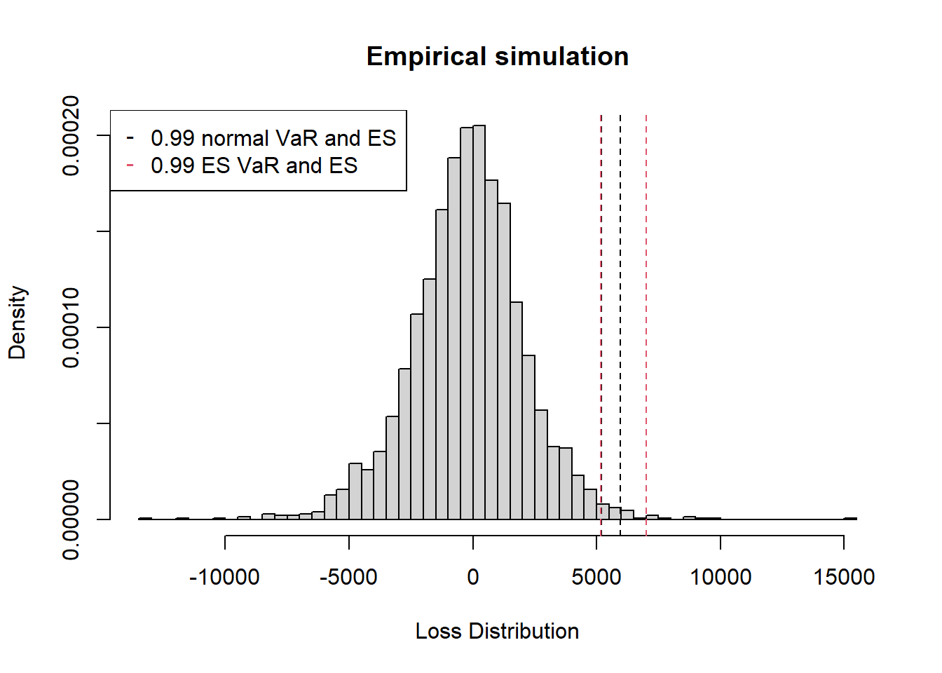
## [1,] 5965.354

Empirical simulation.

Instead of assuming the underlying random variables, such as the risk factors in our case, we can utilize the empirical distribution function (EDF). This function is associated with the empirical measure of a sample. For example, when considering losses over the entire sample period, it is theoretically expected to follow some normal distribution. We can visually validate this assumption by creating a quantile-quantile plot for the losses.

qqnorm(loss)

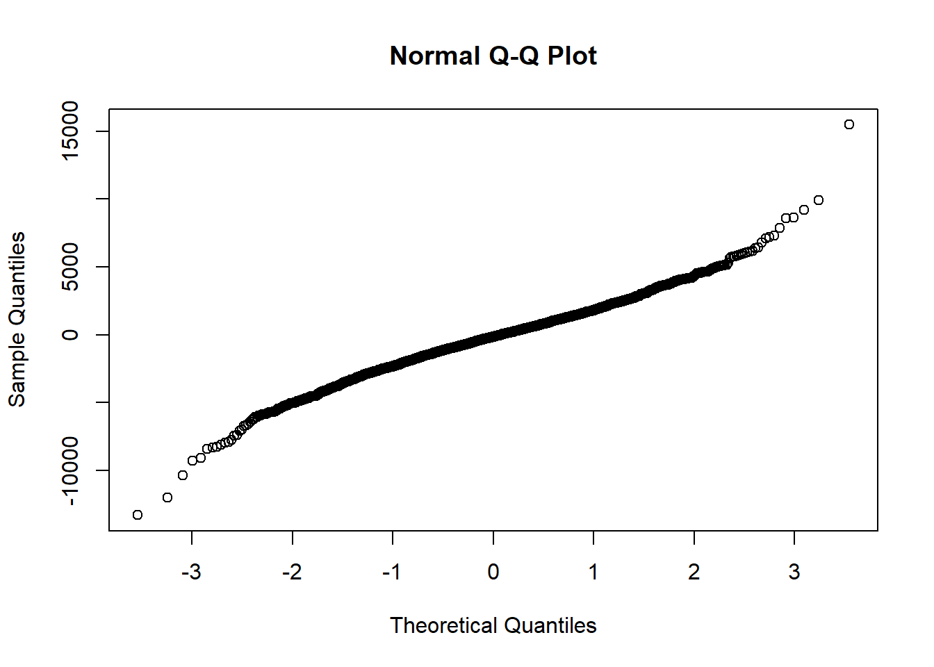
If obvious patterns or evidence are reflected in the QQ plot, indicating significant deviations of losses from a normal distribution, it is advisable to rely on the empirical results.

# Find the VaR of the portfolio loss with EDF.
VaR.hs <- quantile(loss, alpha)
VaR.hs

##      99% 
## 5171.709

# Find the ES of the portfolio loss with EDF.
ES.hs <- mean(loss[loss > VaR.hs])
ES.hs

## [1] 7015.152

Present the empirical results and compare with the normal case by plotting a histogram.

hist(loss,nclass=100, prob=TRUE,
     xlab="Loss Distribution",
     main="Empirical simulation")
abline(v=c(VaR.normal,ES.normal),col=1,lty=2);
abline(v=c(VaR.hs,ES.hs),col=2,lty=2)
legendnames <- c(paste(alpha,"normal VaR and ES"),paste(alpha,"ES VaR and ES"))
legend("topleft", legend = legendnames, col=1:2, pch="-")