Calibration of Copulas

Copula functions play a vital role in financial applications, helping to assess the dependence structure of asset returns within a portfolio.

Within this section, we aim to describe some simple statistical procedures for calibrating the copula functions: normal (standard), t (both-tailed), Gumbel (upper-tailed) and Clayton (lower tailed) to (1) simulated data and (2) financial market data, for instance, FTSE 100 Stock Market Index, Swiss Market Index and Sterling Exchange Rates (USD, EUR, JPY, CHF).

To complete tasks in this section, we only need the QRM library.

library("QRM")

Copula Fitting from Simulated Data

First of all, we prepare some data to be used for calibrating copula functions.

Generation of pseudo-copula data

rm(list=ls(all=TRUE))

Set up parameters

Set \(n\): number of observation (sample size).

nObs <- 5000

Set \(d\): number of dimensions of the FOUR copulas.

normNVar <- 4     # Normal
tNVar <- 4        # T
gumbNVar <- 4     # Gumbel
clayNVar <- 4     # Clayton

Construct the covariance matrices for the normal and \(t\) distributions, with specifying an arbitrary value as the correlation between any two variables.

# correlation parameter
cor.par <- 0.7

For normal: equicorr(normNVar,cor.par) constructs an equal correlation matrix with dimension normNVar = 4 and correlation cor.par = 0.7, the result of which is equivalent to (1-cor.par)*diag(normNVar) + array(cor.par,c(normNVar,normNVar)), the formula given in the lecture slides.

normSigma <- equicorr(normNVar,cor.par) 
normSigma

##      [,1] [,2] [,3] [,4]
## [1,]  1.0  0.7  0.7  0.7
## [2,]  0.7  1.0  0.7  0.7
## [3,]  0.7  0.7  1.0  0.7
## [4,]  0.7  0.7  0.7  1.0

For t: it is equivalent to (1-cor.par)*diag(tNVar) + array(cor.par,c(tNVar,tNVar)).

tSigma <- equicorr(tNVar,cor.par)   
tSigma

##      [,1] [,2] [,3] [,4]
## [1,]  1.0  0.7  0.7  0.7
## [2,]  0.7  1.0  0.7  0.7
## [3,]  0.7  0.7  1.0  0.7
## [4,]  0.7  0.7  0.7  1.0

Other parameters for setting up the copula functions.

# degree of freedom for t
t.dof <- 4
# theta paramaters for Gumbel and Clayton
thetaGumb <- 2
thetaClay <- 2.2

# for displaying contour charts
distribution.limits <- c(0.01,0.99)
Sigma.contour <- equicorr(2,0.5)
threed.limits <- c(-3,3)

Method A: Pseudo-copula

Simply put, this method involves generating ‘pseudo-copula’ data (cumulative probability) by simulating random data and calculating the corresponding cumulative probabilities for the copula.

Simulate multivariate data.

By normal with mean zero and covariance normSigma.

set.seed(1)
normData <- rmnorm(nObs,mu=array(0,normNVar),normSigma) 
head(normData,3)

##            [,1]      [,2]       [,3]        [,4]
## [1,] -0.6264538 -1.521425 -1.4078727 -1.17025139
## [2,]  0.1836433  0.577847 -0.3740229  0.04657662
## [3,] -0.8356286 -1.783410 -1.7522544 -1.56416507

By student’s \(t\) with t.dof degrees of freedom, mean zero and dispersion matrix tSigma.

set.seed(2) 
tData <- rmt(nObs,t.dof,mu=array(0,tNVar),tSigma)
head(tData,3)

##           [,1]       [,2]       [,3]      [,4]
## [1,]  1.313148  1.5287090  0.7784795  1.470350
## [2,] -1.926051 -0.3230757 -1.3793929 -1.847529
## [3,] -2.787800 -2.8804411 -1.7511055 -1.254295

Compute the corresponding cumulative probabilities (the pseudo-copula data).

We apply the normal/\(t\) distribution function function (DF) to the columns of the data we simulated from the normal/\(t\) distributions.

Note: here we consider the simulated data from a known distribution and use pnorm() and tnorm, respectively. In the next section, we use the empirical distribution function edf() instead because we look at real data with unknown distribution.

To efficiently apply the function pnorm() to every column of normData, we utilise the R built-in function apply(). Check ?apply for the usage of this function.

gaussCopulaData <- apply(normData,2,pnorm)   
head(gaussCopulaData,3)

##           [,1]       [,2]       [,3]      [,4]
## [1,] 0.2655087 0.06407663 0.07958439 0.1209499
## [2,] 0.5728534 0.71831629 0.35419362 0.5185747
## [3,] 0.2016819 0.03725977 0.03986503 0.0588894

Apply the same function to tData.

tCopulaData <- apply(tData,2,pt,df=t.dof)
head(tCopulaData,3)

##            [,1]       [,2]       [,3]       [,4]
## [1,] 0.87030186 0.89946758 0.76011628 0.89229117
## [2,] 0.06319415 0.38141092 0.11993661 0.06919261
## [3,] 0.02471149 0.02249657 0.07740809 0.13901519

Display the pseudo-copula data.

pairs(gaussCopulaData)

pairs(tCopulaData)

hist(gaussCopulaData[,4])  #should be very much like Uniform

Bivariate visualization: contour plots of bivariate Gaussian or \(t\) densities.

BiDensPlot(func=dcopula.gauss, xpts=distribution.limits, ypts=distribution.limits,
           Sigma=Sigma.contour)

BiDensPlot(func=dcopula.t, xpts=distribution.limits, ypts=distribution.limits,
           df=t.dof,Sigma=Sigma.contour)

Method B: Reverse the procedures of Method A

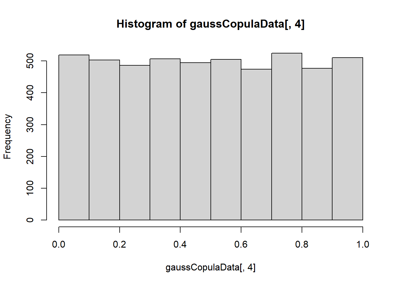
Compute cumulative probabilities from the copula functions.

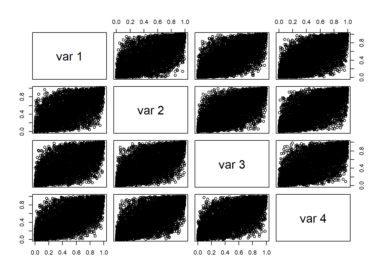
Generate sample data from the four copula functions by using the function rcopula.CopulaName(). See illustrations below.

\((U_{1,i}, \dots, U_{4,i}) \sim \mathcal{C}^{Ga}_{P=normSigma}\), for \(i=1, ... ,nObs\).

set.seed(3)
u.normc <- rcopula.gauss(nObs,normSigma)
head(u.normc,3)

##           [,1]       [,2]      [,3]      [,4]
## [1,] 0.1680415 0.32726624 0.1467003 0.1569128
## [2,] 0.3849423 0.94398745 0.6767277 0.8268005
## [3,] 0.6021007 0.09866179 0.2924065 0.1541135

\((U_{1,i}, \dots, U_{4,i}) \sim \mathcal{C}^{Gu}_{\theta=thetaGumb}\), \(i=1, ... ,nObs\).

set.seed(4)
u.gumbc <- rcopula.gumbel(nObs,theta=thetaGumb, d=gumbNVar) 
head(u.gumbc,3)

##           [,1]      [,2]      [,3]      [,4]
## [1,] 0.2457526 0.3603885 0.5026453 0.3989128
## [2,] 0.6645462 0.7253971 0.8439990 0.7858096
## [3,] 0.9522377 0.9470578 0.9727424 0.9941587

\((U_{1,i}, \dots, U_{4,i}) \sim \mathcal{C}^{Cl}_{\theta=thetaClay}\), \(i=1, ... ,nObs\).

set.seed(5)
u.clayc <- rcopula.clayton(nObs, theta=thetaClay, d=clayNVar)  
head(u.clayc,3)

##           [,1]      [,2]      [,3]      [,4]
## [1,] 0.3060311 0.2565782 0.2812887 0.2926362
## [2,] 0.7084404 0.8768012 0.6547532 0.4869972
## [3,] 0.8422283 0.9538730 0.5045568 0.4018928

\((U_{1,i}, \dots, U_{4,i}) \sim \mathcal{C}^{t}_{P=tSigma}\), \(i=1, ... ,nObs\).

set.seed(6)
u.tc <- rcopula.t(nObs, df=t.dof, tSigma)      
head(u.tc,3)

##           [,1]      [,2]      [,3]      [,4]
## [1,] 0.7377204 0.8466876 0.8044272 0.8259748
## [2,] 0.8532993 0.9389583 0.6453806 0.9106730
## [3,] 0.2578326 0.2318692 0.3789596 0.1862297

Plots of simulated data (Column 1 vs Column 2).

par(mfrow=c(2,2)) # For 2x2 plots in one window
plot(u.normc)
plot(u.gumbc)
plot(u.clayc)
plot(u.tc)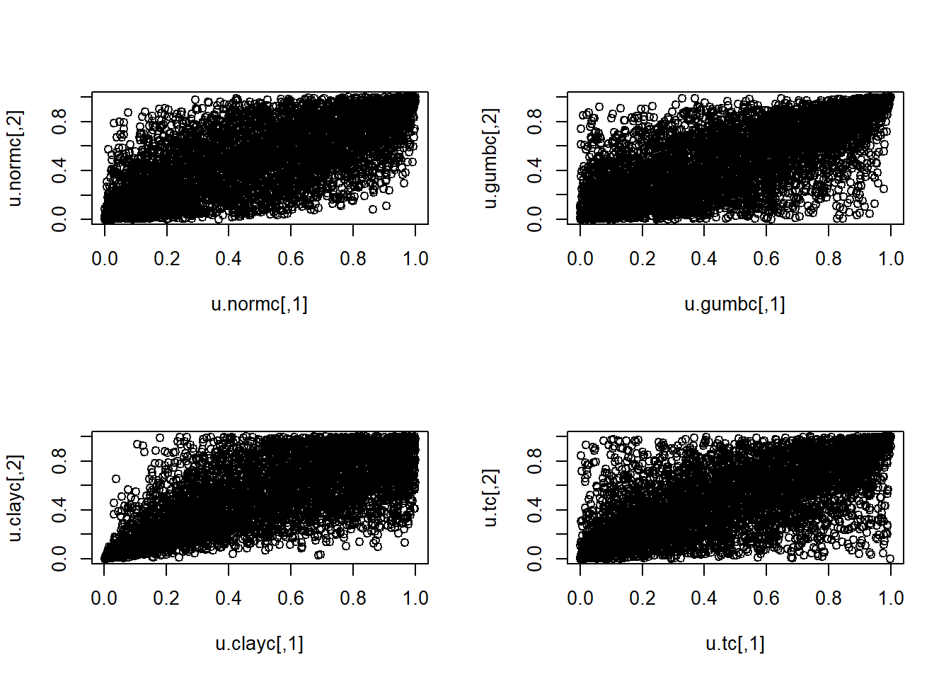

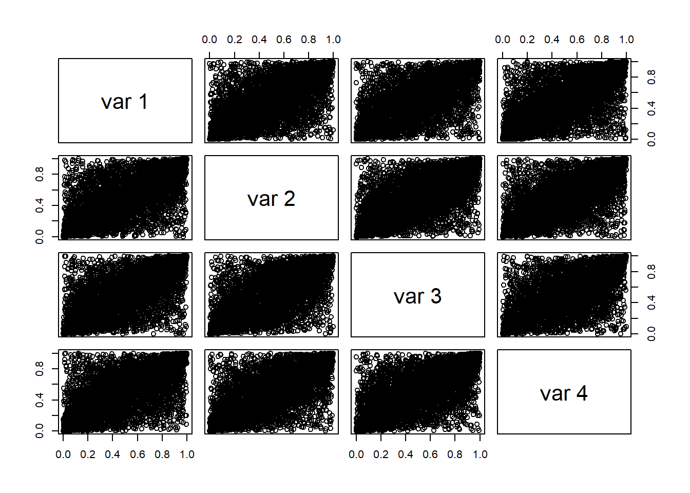
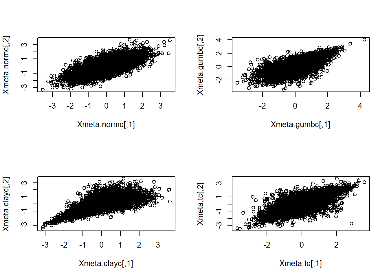
Meta distributions.

If we use a different quantile distribution (\(F^{-1}\)) than that associated with the copula which generated the data, we are creating a ‘Meta distribution’. In the following we use quantiles for ‘normal marginals’ (via the normal quantile function) with probabilities generated by the Gumbel, Clayton, and \(t\) copulas. The resulting data values are all known as ‘meta-Gaussian’ distributions.

First, map to \(N(0,1)\) margins (meta-copula data), which results in multivariate normal again.

Xmeta.normc <- qnorm(u.normc)

For the rest we do: \[ \mathbb{P}\left( \Phi^{-1}(u_1) < x_1, \dots,\Phi^{-1}(u_4) < x_4 \right) = P\left( U_1 < \Phi(x_1), \dots, U_4 < \Phi(x_4) \right), \] i.e., the Copula of \(U\) with normal marginals.

# Gumbel copula with normal marginals
Xmeta.gumbc <- qnorm(u.gumbc)  
head(Xmeta.gumbc,3)

##            [,1]       [,2]        [,3]       [,4]
## [1,] -0.6879167 -0.3574206 0.006630794 -0.2561621
## [2,]  0.4249027  0.5989507 1.011029986  0.7919656
## [3,]  1.6669484  1.6169720 1.922720655  2.5215869

# Clayton copula with normal marginals
Xmeta.clayc <- qnorm(u.clayc) 
head(Xmeta.clayc,3)

##            [,1]       [,2]       [,3]        [,4]
## [1,] -0.5071320 -0.6539308 -0.5790176 -0.54569957
## [2,]  0.5488343  1.1591435  0.3981853 -0.03259883
## [3,]  1.0036584  1.6836259  0.0114224 -0.24845076

# t copula with normal marginals
Xmeta.tc <- qnorm(u.tc)   
head(Xmeta.tc,3)

##            [,1]      [,2]       [,3]       [,4]
## [1,]  0.6363332  1.022330  0.8575417  0.9383776
## [2,]  1.0506892  1.546088  0.3728785  1.3449112
## [3,] -0.6500419 -0.732705 -0.3082145 -0.8918761

Plots of simulated data (Column 1 vs Column 2).

par(mfrow=c(2,2))
plot(Xmeta.normc)
plot(Xmeta.gumbc)
plot(Xmeta.clayc)
plot(Xmeta.tc)

Illustrate in 3D using BiDensPlot with self-defined functions.

BiDensPlot()’s first argument is a function evaluating a \(n \times 2\) matrix, such as

normal.metagumbel <- function(x,theta){
    exp(dcopula.gumbel(apply(x,2,pnorm),theta,log=TRUE) +
        apply(log(apply(x,2,dnorm)),1,sum))
}
normal.metaclayton <- function(x,theta){
    exp(dcopula.clayton(apply(x,2,pnorm),theta,log=TRUE) +
        apply(log(apply(x,2,dnorm)),1,sum))
}
normal.metat <- function(x,df,Sigma){
    exp(dcopula.t(apply(x,2,pnorm),df,Sigma,log=TRUE) +
        apply(log(apply(x,2,dnorm)),1,sum))
}

The perspective plots are given by:

par(mfrow=c(1,2))
BiDensPlot(dmnorm,xpts=threed.limits,ypts=threed.limits,mu=c(0,0),
           Sigma=Sigma.contour) 
BiDensPlot(normal.metagumbel,xpts=threed.limits,ypts=threed.limits,
           npts=80,theta=thetaGumb)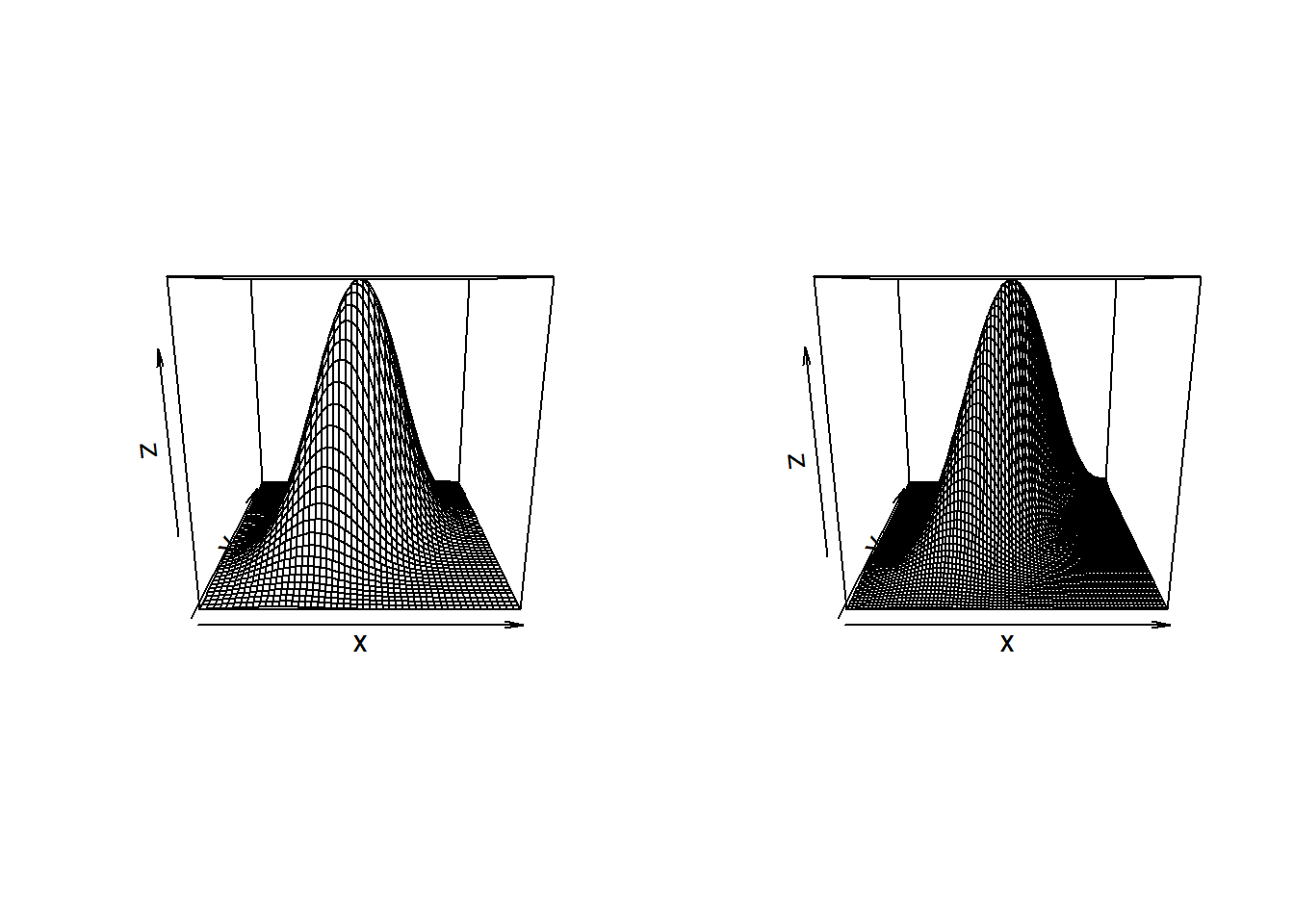

BiDensPlot(normal.metaclayton,xpts=threed.limits,ypts=threed.limits,
           npts=80,theta=thetaClay) 
BiDensPlot(normal.metat,xpts=threed.limits,ypts=threed.limits,
           npts=80,df=t.dof,Sigma=Sigma.contour)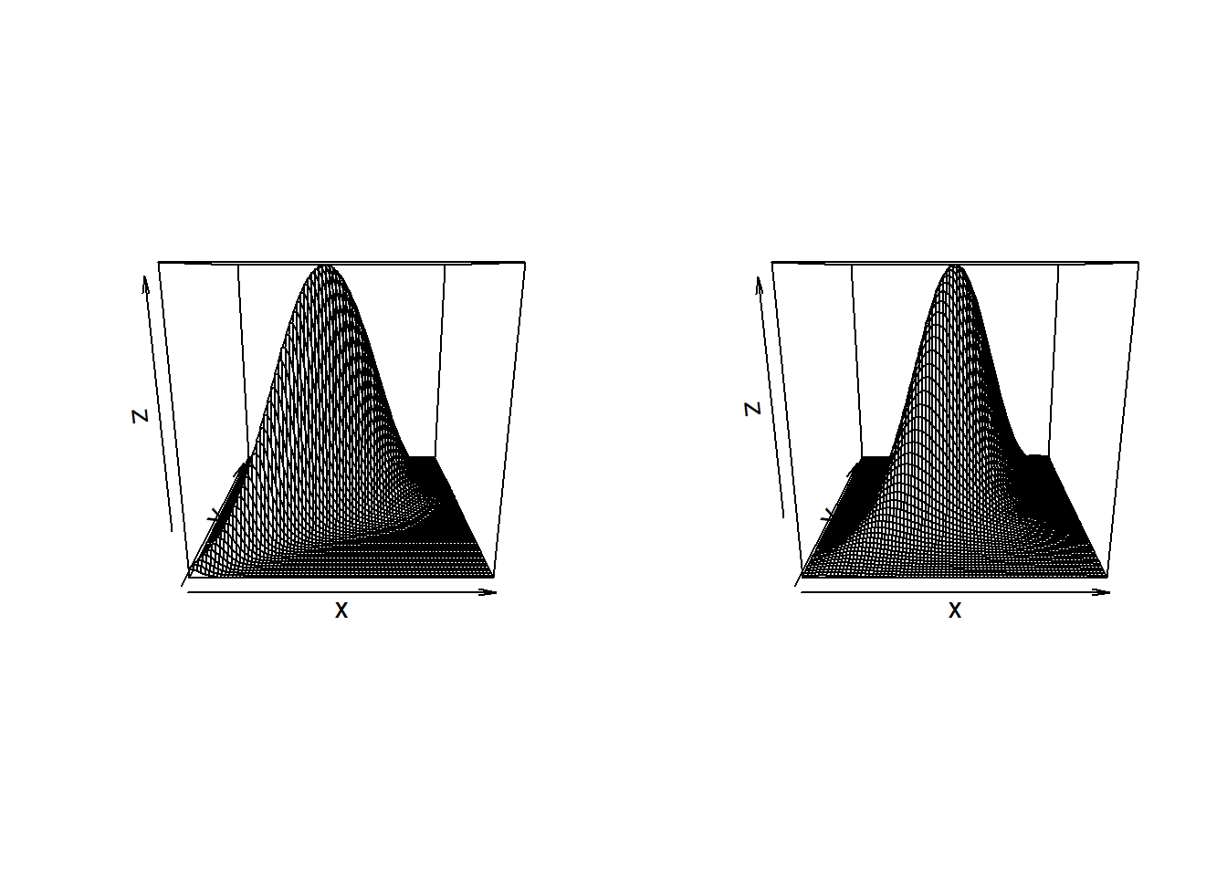

and the contour plots are by

par(mfrow=c(2,2)) 
BiDensPlot(dmnorm,type="contour",xpts=threed.limits,ypts=threed.limits,
           mu=c(0,0), Sigma=Sigma.contour)
BiDensPlot(normal.metagumbel,type="contour",xpts=threed.limits,
           ypts=threed.limits, npts=80,theta=thetaGumb)
BiDensPlot(normal.metaclayton,type="contour",xpts=threed.limits,
           ypts=threed.limits, npts=80,theta=thetaClay)
BiDensPlot(normal.metat,type="contour",xpts=threed.limits,
           ypts=threed.limits, npts=80,df=t.dof,Sigma=Sigma.contour)

Copula Fitting from Empirical Data

Load data.

We require three sources of data from FTSE 100 Stock Market Index, Swiss Market Index and Sterling Exchange Rates (USD, EUR, JPY, CHF), which can be accessed by the way below:

# FTSE 100 Stock Market Index, daily from 1990-01-02 to 2004-03-25
data(ftse100)
# Swiss Market Index, daily from 1990-11-09 to 2004-03-25
data(smi)  
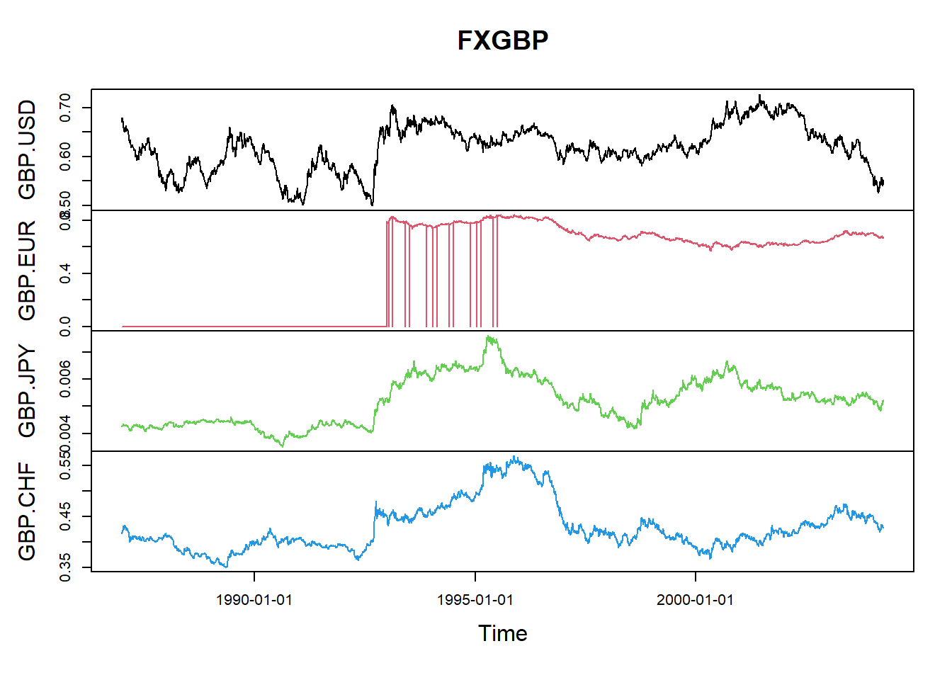
# Sterling Exchange Rates (USD, EUR, JPY, CHF), 
# daily from 1987-01-02 to 2004-03-31
data(FXGBP)

Merge and transform.

We construct a bivariate time series from FTSE100 and SMI data between 1990-11-09 and 2004-03-25.

Note that the number of observations between these dates differs due to holidays, but the function alignDailySeries returns from a daily time series with missing holidays a weekly aligned daily timeSeries object.
```
ftseDataInSMIInterval <- window(ftse100, "1990-11-09", "2004-03-25")
ftseDataAligned <- alignDailySeries(ftseDataInSMIInterval, method="before")
smiDataAligned <- alignDailySeries(smi, method="before")
stockIndexPrices <- merge(ftseDataAligned,smiDataAligned)
plot(stockIndexPrices)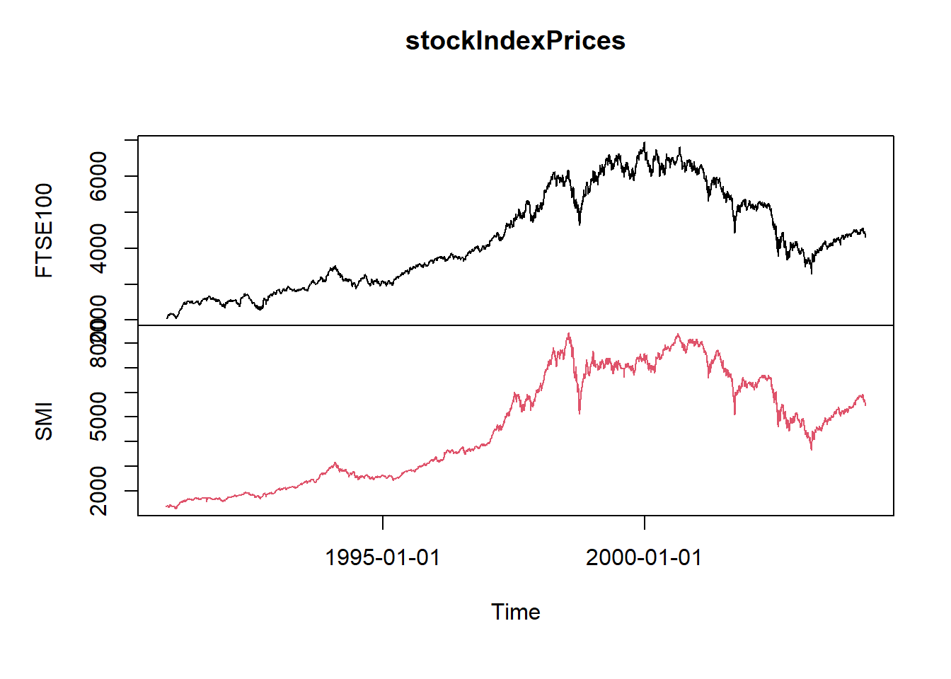
```

Calculate the log returns.

stockIndexLogPrices <- log(stockIndexPrices)
stockIndexReturns <- diff(stockIndexLogPrices)
head(stockIndexReturns,5)

## GMT
##                 FTSE100          SMI
## 1990-11-09           NA           NA
## 1990-11-12  0.005522311  0.014599844
## 1990-11-13  0.001996154  0.005455783
## 1990-11-14 -0.004875680 -0.003468416
## 1990-11-15  0.006819315 -0.003267048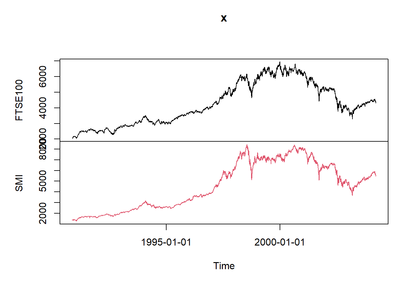

plot(stockIndexReturns)

Restrict to an interval of 10 years.

stockIndexReturns <- window(stockIndexReturns, "1994-01-01", "2003-12-31")
head(stockIndexReturns,5)

## GMT
##                 FTSE100         SMI
## 1994-01-03  0.000000000 0.012966690
## 1994-01-04 -0.002900294 0.001000767
## 1994-01-05 -0.008633317 0.003395137
## 1994-01-06  0.007018400 0.004145049
## 1994-01-07  0.012556743 0.006925235

plot(stockIndexReturns)

Transform into a matrix object.

Delete rows where both indices have zero return: these correspond to the holidays in both countries, e.g. 25 December.

X <- as.matrix(stockIndexReturns)
X <- X[X[,1]!=0 & X[,2] !=0,]
head(X,5)

##                 FTSE100          SMI
## 1994-01-04 -0.002900294  0.001000767
## 1994-01-05 -0.008633317  0.003395137
## 1994-01-06  0.007018400  0.004145049
## 1994-01-07  0.012556743  0.006925235
## 1994-01-10 -0.001568263 -0.008912715

Construct pseudo copula data.

The apply function below uses the edf() empirical distribution function for the columns of the data. Setting adjust=1 inside the edf function allows the adjustment of denominator to be \((n+1)\).

copulaX <- apply(X,2,edf,adjust=1)
head(copulaX,5)

##        FTSE100       SMI
## [1,] 0.3638968 0.5186246
## [2,] 0.1817438 0.6221858
## [3,] 0.7670896 0.6528858
## [4,] 0.8915268 0.7425297
## [5,] 0.4126074 0.1866558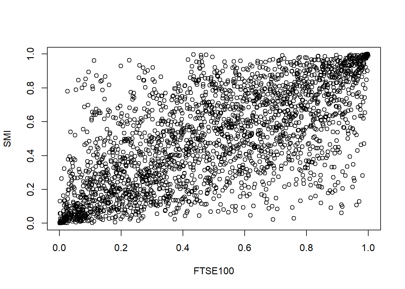

plot(copulaX)

Compare various bivariate models.

Gaussian copula fit

copulaXGauss <- fit.gausscopula(copulaX)
copulaXGauss

## $P
##           [,1]      [,2]
## [1,] 1.0000000 0.7081993
## [2,] 0.7081993 1.0000000
## 
## $converged
## [1] TRUE
## 
## $ll.max
## [1] 845.5582
## 
## $fit
## $fit$par
## [1] 1.003097
## 
## $fit$objective
## [1] -845.5582
## 
## $fit$convergence
## [1] 0
## 
## $fit$iterations
## [1] 4
## 
## $fit$evaluations
## function gradient 
##        6        7 
## 
## $fit$message
## [1] "relative convergence (4)"

Student’s t copula

copulaXt <- fit.tcopula(copulaX)
copulaXt

## $P
##           [,1]      [,2]
## [1,] 1.0000000 0.7051436
## [2,] 0.7051436 1.0000000
## 
## $nu
## [1] 4.483919
## 
## $converged
## [1] TRUE
## 
## $ll.max
## [1] 898.4885
## 
## $fit
## $fit$par
## [1] 4.4839193 0.9944702
## 
## $fit$objective
## [1] -898.4885
## 
## $fit$convergence
## [1] 0
## 
## $fit$iterations
## [1] 7
## 
## $fit$evaluations
## function gradient 
##        9       21 
## 
## $fit$message
## [1] "relative convergence (4)"

2-dimensional Archimedian copulas (Gumbel and Clayton)

# Gumbel copula fit
copulaXGumb <- fit.AC(copulaX,"gumbel")
copulaXGumb

## $ll.max
## [1] 808.2028
## 
## $theta
## [1] 1.91942
## 
## $se
## [1] 0.0315802
## 
## $converged
## [1] TRUE
## 
## $fit
## $fit$par
## [1] 1.91942
## 
## $fit$objective
## [1] -808.2028
## 
## $fit$convergence
## [1] 0
## 
## $fit$iterations
## [1] 4
## 
## $fit$evaluations
## function gradient 
##        6        6 
## 
## $fit$message
## [1] "relative convergence (4)"

# Clayton copula fit
copulaXClay <- fit.AC(copulaX,"clayton")
copulaXClay

## $ll.max
## [1] 742.7924
## 
## $theta
## [1] 1.468476
## 
## $se
## [1] 0.04745088
## 
## $converged
## [1] TRUE
## 
## $fit
## $fit$par
## [1] 1.468476
## 
## $fit$objective
## [1] -742.7924
## 
## $fit$convergence
## [1] 0
## 
## $fit$iterations
## [1] 6
## 
## $fit$evaluations
## function gradient 
##        7        9 
## 
## $fit$message
## [1] "relative convergence (4)"

Calculate Spearman’s rank correlation and Kendall’s tau.

Spearman(copulaX)

##           FTSE100       SMI
## FTSE100 1.0000000 0.6720367
## SMI     0.6720367 1.0000000

sin(pi*Kendall(copulaX)/2)

##           FTSE100       SMI
## FTSE100 1.0000000 0.7011095
## SMI     0.7011095 1.0000000

c(copulaXGauss$ll.max, copulaXt$ll.max, 
  copulaXGumb$ll.max, copulaXClay$ll.max)

## [1] 845.5582 898.4885 808.2028 742.7924

Multivariate fitting using Gauss and \(t\) copula on GBP crosses.

Data preparation.
```
plot(FXGBP)
```

Calculate returns and restrict time period.

gbpLogPrices <- log(FXGBP) 
gbpReturns <- diff(gbpLogPrices)
gbpReturns <- window(gbpReturns, "1997-01-01", "2003-12-31")
head(gbpReturns,5)

## GMT
##                 GBP.USD      GBP.EUR       GBP.JPY      GBP.CHF
## 1997-01-02  0.015294456  0.012534003  0.0173743094  0.011735753
## 1997-01-03 -0.002397637 -0.014306279 -0.0091998770 -0.014375276
## 1997-01-06  0.002970867  0.002779710  0.0072690544  0.004105463
## 1997-01-07 -0.005679336 -0.004459453 -0.0017976479 -0.003025860
## 1997-01-08  0.003924891 -0.003587423 -0.0002934014 -0.004233200

plot(gbpReturns)

Transform into a matrix object and delete rows where all currencies have zero return.

Y <- as.matrix(gbpReturns)
Y <- Y[Y[,1]!=0 & Y[,2] !=0,]
head(Y,5)

##                 GBP.USD      GBP.EUR       GBP.JPY      GBP.CHF
## 1997-01-02  0.015294456  0.012534003  0.0173743094  0.011735753
## 1997-01-03 -0.002397637 -0.014306279 -0.0091998770 -0.014375276
## 1997-01-06  0.002970867  0.002779710  0.0072690544  0.004105463
## 1997-01-07 -0.005679336 -0.004459453 -0.0017976479 -0.003025860
## 1997-01-08  0.003924891 -0.003587423 -0.0002934014 -0.004233200

Display scatter plots of all data pairs (e.g GBP/USD, GBP/EUR, GBP/JPY, GBP/CHF).
```
pairs(Y)
```

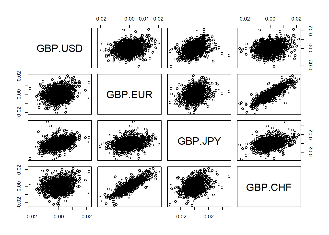
Construct pseudo copula data.

copulaY <- apply(Y,2,edf,adjust=TRUE)
head(copulaY,5)

##        GBP.USD     GBP.EUR    GBP.JPY     GBP.CHF
## [1,] 0.9977143 0.984000000 0.97714286 0.973714286
## [2,] 0.2874286 0.005714286 0.09714286 0.004571429
## [3,] 0.7577143 0.749714286 0.85200000 0.794857143
## [4,] 0.1074286 0.160000000 0.39485714 0.269714286
## [5,] 0.8137143 0.222285714 0.49371429 0.194285714

Display scatter plots of all data pairs (e.g GBP/USD, GBP/EUR, GBP/JPY, GBP/CHF) generated from the Empirical Distribution Function edf.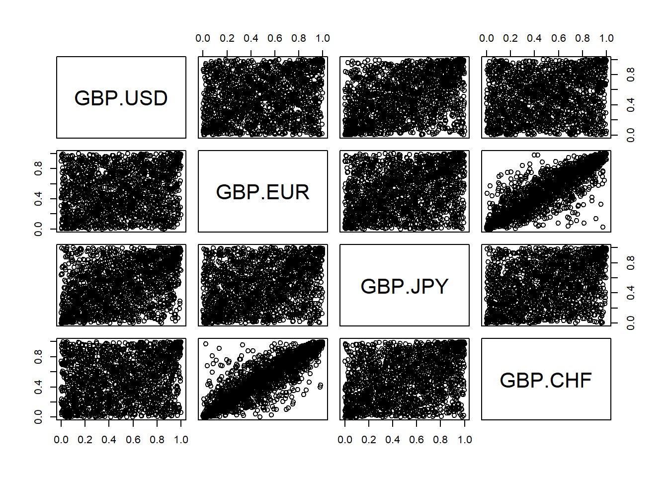
```
pairs(copulaY)
```

Fit \(t\) copula using rank correlations to the ECDF data.

copulaYt <- fit.tcopula(copulaY, method="Kendall")
copulaYt

## $P
##           GBP.USD   GBP.EUR   GBP.JPY   GBP.CHF
## GBP.USD 1.0000000 0.1842613 0.4181550 0.1595692
## GBP.EUR 0.1842613 1.0000000 0.2905980 0.8830913
## GBP.JPY 0.4181550 0.2905980 1.0000000 0.3147264
## GBP.CHF 0.1595692 0.8830913 0.3147264 1.0000000
## 
## $nu
## [1] 6.577836
## 
## $converged
## [1] TRUE
## 
## $ll.max
## [1] 1620.814
## 
## $fit
## $fit$par
## [1] 6.577836
## 
## $fit$objective
## [1] -1620.814
## 
## $fit$convergence
## [1] 0
## 
## $fit$iterations
## [1] 6
## 
## $fit$evaluations
## function gradient 
##        7        9 
## 
## $fit$message
## [1] "relative convergence (4)"

Estimate Spearman rank correlations.

copulaYcorr <- Spearman(copulaY)
copulaYcorr

##           GBP.USD   GBP.EUR   GBP.JPY   GBP.CHF
## GBP.USD 1.0000000 0.1727292 0.3937847 0.1490981
## GBP.EUR 0.1727292 1.0000000 0.2718689 0.8608703
## GBP.JPY 0.3937847 0.2718689 1.0000000 0.2971055
## GBP.CHF 0.1490981 0.8608703 0.2971055 1.0000000

Function dcopula.gauss provides a vector of density values, used for evaluating the Gauss copula, generating random variates and fitting.

sum(dcopula.gauss(copulaY,copulaYcorr,log=TRUE))

## [1] 1485.325