11 时间序列回归

library(cmdstanr)
library(zoo)
library(xts) # xts 依赖 zoo
library(fGarch)
library(INLA)
library(mgcv)
library(tensorflow)
library(ggplot2)
library(bayesplot)

11.1 随机波动率模型

随机波动率模型主要用于股票时间序列数据建模。本节以美团股价数据为例介绍随机波动率模型，并分别以 Stan 框架和 fGarch 包拟合模型。

# 美团上市至 2023-07-15
meituan <- readRDS(file = "data/meituan.rds")
library(zoo)
library(xts)
library(ggplot2)
autoplot(meituan[, "3690.HK.Adjusted"]) +
  theme_classic() +
  labs(x = "日期", y = "股价")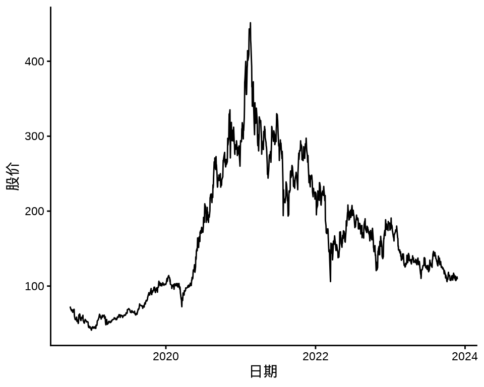

对数收益率的计算公式如下：

$对数收益率 = \ln (今日收盘价 / 昨日收盘价) = \ln (1 + 普通收益率)$

下图给出股价对数收益率变化和股价对数收益率的分布，可以看出在不同时间段，收益率波动幅度是不同的，美团股价对数收益率的分布可以看作正态分布。

meituan_log_return <- diff(log(meituan[, "3690.HK.Adjusted"]))[-1]
autoplot(meituan_log_return) +
  theme_classic() +
  labs(x = "日期", y = "对数收益率")
ggplot(data = meituan_log_return, aes(x = `3690.HK.Adjusted`)) +
  geom_histogram(color = "black", fill = "gray", bins = 30) +
  theme_classic() +
  labs(x = "对数收益率", y = "频数（天数）")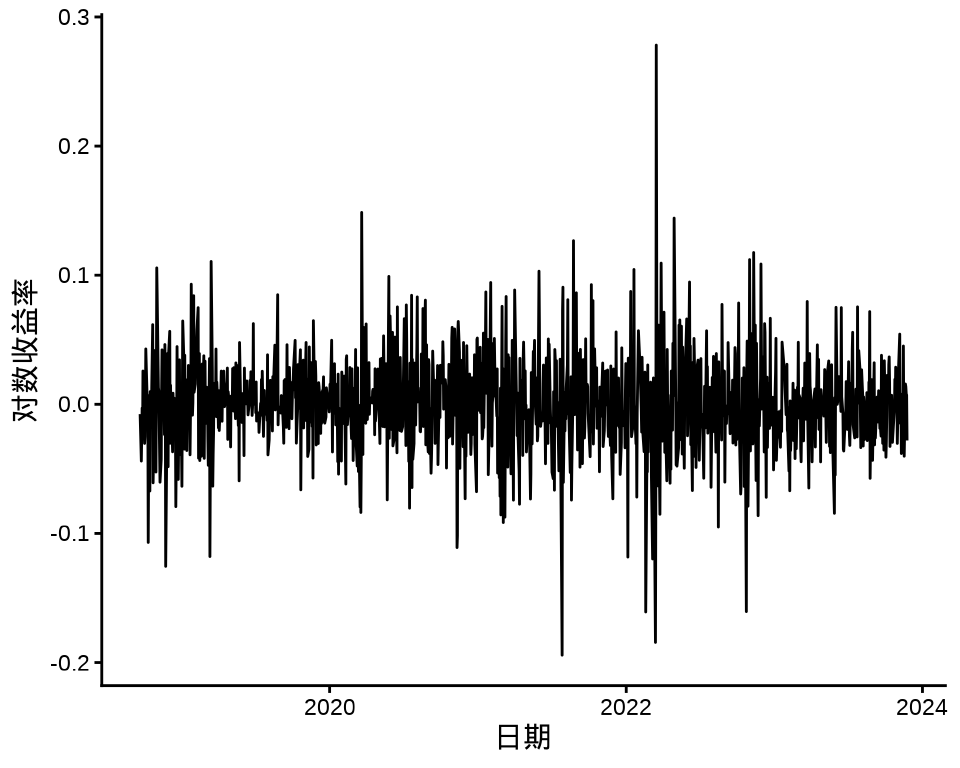

检查对数收益率序列的自相关图

acf(meituan_log_return, main = "")

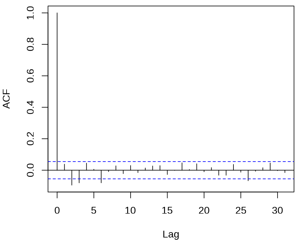
发现，滞后 2、3、6、26 阶都有出界，滞后 17 阶略微出界，其它的自相关都在零水平线的界限内。

Box.test(meituan_log_return, lag = 12, type = "Ljung")

#> 
#>  Box-Ljung test
#> 
#> data:  meituan_log_return
#> X-squared = 35.669, df = 12, p-value = 0.0003661

在 0.05 水平下拒绝了白噪声检验，说明对数收益率序列存在相关性。同理，也注意到对数收益率的绝对值和平方序列都不是独立的，存在相关性。

# ARCH 效应的检验
Box.test((meituan_log_return - mean(meituan_log_return))^2, 
         lag = 12, type = "Ljung")

#> 
#>  Box-Ljung test
#> 
#> data:  (meituan_log_return - mean(meituan_log_return))^2
#> X-squared = 124.54, df = 12, p-value < 2.2e-16

结果高度显著，说明有 ARCH 效应。

11.1.1 Stan 框架

随机波动率模型如下

$\begin{aligned} y_{t} & = ϵ_{t} \exp (h_{t} / 2) \\ h_{t + 1} & = μ + ϕ (h_{t} - μ) + δ_{t} σ \\ h_{1} & \sim normal (μ, \frac{σ}{\sqrt{1 - ϕ^{2}}}) \\ ϵ_{t} & \sim normal (0, 1) \\ δ_{t} & \sim normal (0, 1) \end{aligned}$

其中， $y_{t}$ 表示在时间 $t$ 时股价的回报（对数收益率）， $ϵ_{t}$ 表示股价回报在时间 $t$ 时的白噪声扰/波动， $δ_{t}$ 表示波动率在时间 $t$ 时的波动。 $h_{t}$ 表示对数波动率，带有参数 $μ$ （对数波动率的均值）， $ϕ$ （对数波动率的趋势）。代表波动率的序列 ${h_{t}}$ 假定是平稳 $(| ϕ | < 1)$ 的随机过程， $h_{1}$ 来自平稳的分布（此处为正态分布）， $ϵ_{t}$ 和 $δ_{t}$ 是服从不相关的标准正态分布。

Stan 代码如下

data {
  int<lower=0> T;   // # time points (equally spaced)
  vector[T] y;      // mean corrected return at time t
}
parameters {
  real mu;                     // mean log volatility
  real<lower=-1, upper=1> phi; // persistence of volatility
  real<lower=0> sigma;         // white noise shock scale
  vector[T] h_std;             // std log volatility time t
}
transformed parameters {
  vector[T] h = h_std * sigma;  // now h ~ normal(0, sigma)
  h[1] /= sqrt(1 - phi * phi);  // rescale h[1]
  h += mu;
  for (t in 2:T) {
    h[t] += phi * (h[t - 1] - mu);
  }
}
model {
  phi ~ uniform(-1, 1);
  sigma ~ cauchy(0, 5);
  mu ~ cauchy(0, 10);
  
  h_std ~ std_normal();
  y ~ normal(0, exp(h / 2));
}

编译和拟合模型

library(cmdstanr)
# 编译模型
mod_volatility_normal <- cmdstan_model(
  stan_file = "code/stochastic_volatility_models.stan",
  compile = TRUE, cpp_options = list(stan_threads = TRUE)
)
# 准备数据
mdata = list(T = 1274, y = as.vector(meituan_log_return))
# 拟合模型
fit_volatility_normal <- mod_volatility_normal$sample(
  data = mdata,
  chains = 2,
  parallel_chains = 2,
  iter_warmup = 1000, 
  iter_sampling = 1000, 
  threads_per_chain = 2, 
  seed = 20232023,
  show_messages = FALSE,
  refresh = 0
)
# 输出结果
fit_volatility_normal$summary(c("mu", "phi", "sigma", "lp__"))

#> # A tibble: 4 × 10
#>   variable     mean   median      sd     mad       q5      q95  rhat ess_bulk
#>   <chr>       <dbl>    <dbl>   <dbl>   <dbl>    <dbl>    <dbl> <dbl>    <dbl>
#> 1 mu         -6.86    -6.86   0.117   0.115    -7.05    -6.66   1.00    1322.
#> 2 phi         0.915    0.922  0.0348  0.0300    0.849    0.960  1.00     374.
#> 3 sigma       0.294    0.286  0.0627  0.0608    0.207    0.405  1.01     366.
#> 4 lp__     3088.    3087.    29.2    28.8    3041.    3136.     1.00     544.
#> # ℹ 1 more variable: ess_tail <dbl>

11.1.2 fGarch 包

《金融时间序列分析讲义》两个波动率建模方法

自回归条件异方差模型（Autoregressive Conditional Heteroskedasticity，简称 ARCH）。
广义自回归条件异方差模型（Generalized Autoregressive Conditional Heteroskedasticity，简称 GARCH ）

确定 ARCH 模型的阶，观察残差的平方的 ACF 和 PACF 。

acf((meituan_log_return - mean(meituan_log_return))^2, main = "")
pacf((meituan_log_return - mean(meituan_log_return))^2, main = "")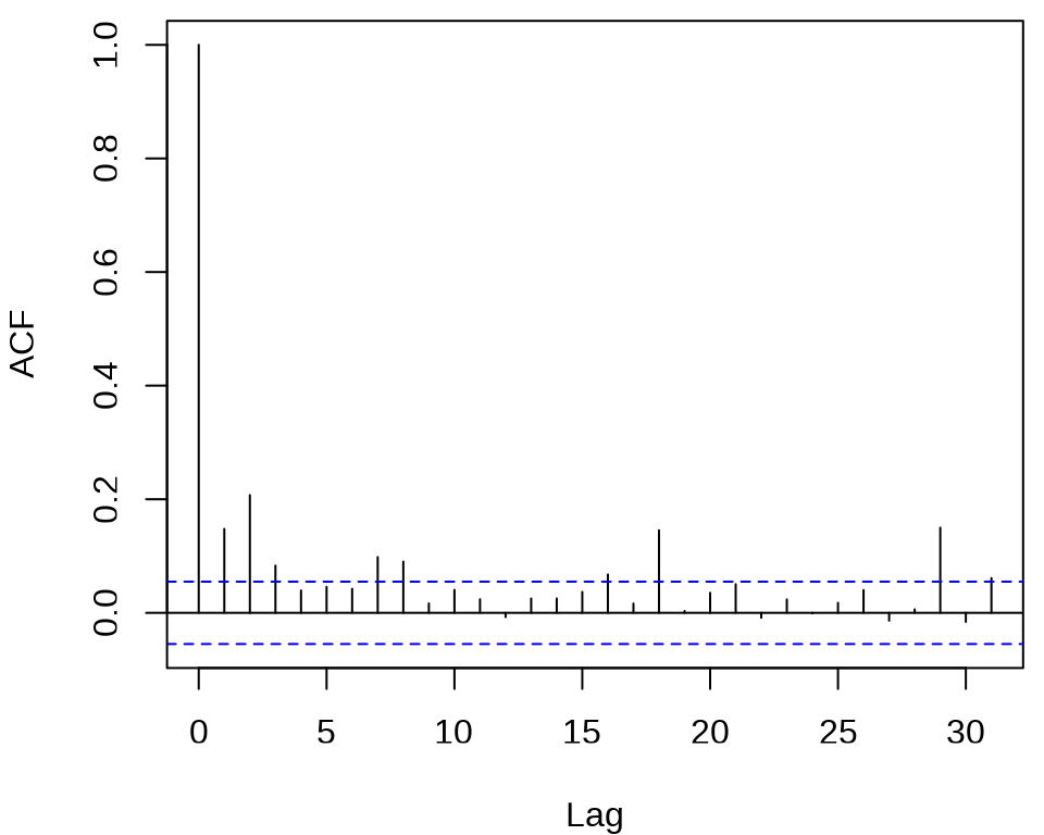

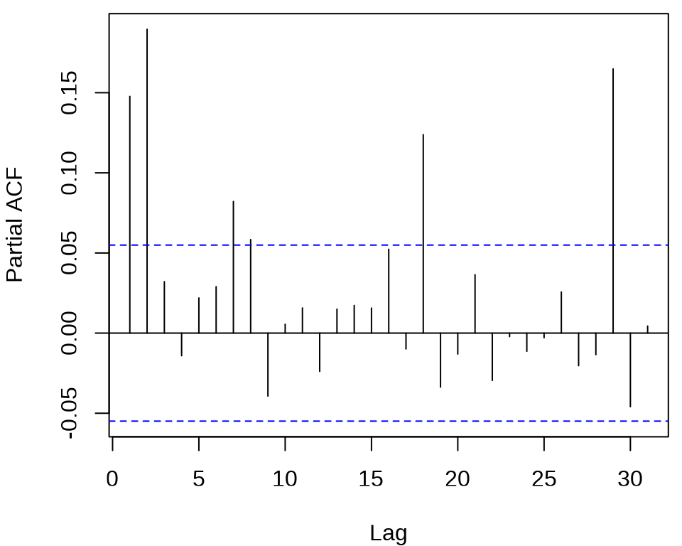
发现 ACF 在滞后 1、2、3 阶比较突出，PACF 在滞后 1、2、16、18、29 阶比较突出。所以下面先来考虑低阶的 ARCH(2) 模型，设 $r_{t}$ 为对数收益率。

$\begin{aligned} r_{t} & = μ + a_{t}, a_{t} = σ_{t} ϵ_{t}, ϵ_{t} \sim N (0, 1) \\ σ_{t}^{2} & = α_{0} + α_{1} a_{t - 1}^{2} + α_{2} a_{t - 2}^{2} . \end{aligned}$

拟合 ARCH 模型，比较模型估计结果，根据系数显著性的结果，采纳 ARCH(2) 模型。

library(fGarch)
meituan_garch1 <- garchFit(
  formula = ~ 1 + garch(2, 0),
  data = meituan_log_return, trace = FALSE, cond.dist = "std"
)
summary(meituan_garch1)

#> 
#> Title:
#>  GARCH Modelling 
#> 
#> Call:
#>  garchFit(formula = ~1 + garch(2, 0), data = meituan_log_return, 
#>     cond.dist = "std", trace = FALSE) 
#> 
#> Mean and Variance Equation:
#>  data ~ 1 + garch(2, 0)
#> <environment: 0x55e487823478>
#>  [data = meituan_log_return]
#> 
#> Conditional Distribution:
#>  std 
#> 
#> Coefficient(s):
#>         mu       omega      alpha1      alpha2       shape  
#> 0.00025765  0.00107291  0.11199514  0.13829052  4.93560791  
#> 
#> Std. Errors:
#>  based on Hessian 
#> 
#> Error Analysis:
#>         Estimate  Std. Error  t value Pr(>|t|)    
#> mu     2.577e-04   8.970e-04    0.287  0.77394    
#> omega  1.073e-03   9.432e-05   11.375  < 2e-16 ***
#> alpha1 1.120e-01   4.292e-02    2.609  0.00907 ** 
#> alpha2 1.383e-01   4.725e-02    2.927  0.00343 ** 
#> shape  4.936e+00   7.008e-01    7.043 1.88e-12 ***
#> ---
#> Signif. codes:  0 '***' 0.001 '**' 0.01 '*' 0.05 '.' 0.1 ' ' 1
#> 
#> Log Likelihood:
#>  2459.345    normalized:  1.930412 
#> 
#> Description:
#>  Mon May  5 23:48:15 2025 by user:  
#> 
#> 
#> Standardised Residuals Tests:
#>                                  Statistic      p-Value
#>  Jarque-Bera Test   R    Chi^2  260.648221 0.000000e+00
#>  Shapiro-Wilk Test  R    W        0.975911 9.515068e-14
#>  Ljung-Box Test     R    Q(10)   21.212805 1.965757e-02
#>  Ljung-Box Test     R    Q(15)   24.773613 5.306761e-02
#>  Ljung-Box Test     R    Q(20)   33.252172 3.165156e-02
#>  Ljung-Box Test     R^2  Q(10)   17.362615 6.671552e-02
#>  Ljung-Box Test     R^2  Q(15)   29.329025 1.458471e-02
#>  Ljung-Box Test     R^2  Q(20)   53.703424 6.400354e-05
#>  LM Arch Test       R    TR^2    19.254099 8.257804e-02
#> 
#> Information Criterion Statistics:
#>       AIC       BIC       SIC      HQIC 
#> -3.852975 -3.832764 -3.853006 -3.845384

函数 garchFit() 的参数 cond.dist 默认值为 "norm" 表示标准正态分布，cond.dist = "std" 表示标准 t 分布。模型均值的估计值接近 0 是符合预期的，且显著性没通过，对数收益率在 0 上下波动。将估计结果代入模型，得到

$\begin{aligned} r_{t} & = - 5.665 \times 10^{- 5} + a_{t}, a_{t} = σ_{t} ϵ_{t}, ϵ_{t} \sim N (0, 1) \\ σ_{t}^{2} & = 1.070 \times 10^{- 3} + 0.1156 a_{t - 1}^{2} + 0.1438 a_{t - 2}^{2} . \end{aligned}$

下面考虑 GARCH(1,1) 模型

$\begin{aligned} r_{t} & = μ + a_{t}, a_{t} = σ_{t} ϵ_{t}, ϵ_{t} \sim N (0, 1) \\ σ_{t}^{2} & = α_{0} + α_{1} a_{t - 1}^{2} + β_{1} σ_{t - 1}^{2} . \end{aligned}$

meituan_garch2 <- garchFit(
  formula = ~ 1 + garch(1, 1),
  data = meituan_log_return, trace = FALSE, cond.dist = "std"
)
summary(meituan_garch2)

#> 
#> Title:
#>  GARCH Modelling 
#> 
#> Call:
#>  garchFit(formula = ~1 + garch(1, 1), data = meituan_log_return, 
#>     cond.dist = "std", trace = FALSE) 
#> 
#> Mean and Variance Equation:
#>  data ~ 1 + garch(1, 1)
#> <environment: 0x55e486770538>
#>  [data = meituan_log_return]
#> 
#> Conditional Distribution:
#>  std 
#> 
#> Coefficient(s):
#>         mu       omega      alpha1       beta1       shape  
#> 2.8294e-04  3.4453e-05  5.9798e-02  9.1678e-01  5.4352e+00  
#> 
#> Std. Errors:
#>  based on Hessian 
#> 
#> Error Analysis:
#>         Estimate  Std. Error  t value Pr(>|t|)    
#> mu     2.829e-04   8.702e-04    0.325  0.74507    
#> omega  3.445e-05   1.937e-05    1.779  0.07525 .  
#> alpha1 5.980e-02   1.855e-02    3.224  0.00127 ** 
#> beta1  9.168e-01   2.784e-02   32.933  < 2e-16 ***
#> shape  5.435e+00   8.137e-01    6.680 2.39e-11 ***
#> ---
#> Signif. codes:  0 '***' 0.001 '**' 0.01 '*' 0.05 '.' 0.1 ' ' 1
#> 
#> Log Likelihood:
#>  2478.473    normalized:  1.945427 
#> 
#> Description:
#>  Mon May  5 23:48:15 2025 by user:  
#> 
#> 
#> Standardised Residuals Tests:
#>                                   Statistic      p-Value
#>  Jarque-Bera Test   R    Chi^2  226.7201557 0.000000e+00
#>  Shapiro-Wilk Test  R    W        0.9781165 5.582407e-13
#>  Ljung-Box Test     R    Q(10)   16.0489321 9.824020e-02
#>  Ljung-Box Test     R    Q(15)   19.6491167 1.858101e-01
#>  Ljung-Box Test     R    Q(20)   27.2460656 1.284820e-01
#>  Ljung-Box Test     R^2  Q(10)    7.8054889 6.478299e-01
#>  Ljung-Box Test     R^2  Q(15)    9.8336965 8.300684e-01
#>  Ljung-Box Test     R^2  Q(20)   24.7640835 2.106061e-01
#>  LM Arch Test       R    TR^2     9.6000051 6.510060e-01
#> 
#> Information Criterion Statistics:
#>       AIC       BIC       SIC      HQIC 
#> -3.883004 -3.862792 -3.883034 -3.875413

波动率的贡献主要来自 $σ_{t - 1}^{2}$ ，其系数 $β_{1}$ 为 0.918。通过对数似然的比较，可以发现 GARCH(1,1) 模型比 ARCH(2) 模型更好。

11.2 贝叶斯可加模型

大规模时间序列回归，观察值是比较多的，可达数十万、数百万，乃至更多。粗粒度时时间跨度往往很长，比如数十年的天粒度数据，细粒度时时间跨度可短可长，比如数年的半小时级数据，总之，需要包含多个季节的数据，各种季节性重复出现。通过时序图可以观察到明显的季节性，而且往往是多种周期不同的季节性混合在一起，有时还包含一定的趋势性。举例来说，比如 2018-2023 年美国旧金山犯罪事件报告数据，事件数量的变化趋势，除了上述季节性因素，特殊事件疫情肯定会影响，数据规模约 200 M 。再比如 2018-2023 年美国境内和跨境旅游业中的航班数据，原始数据非常大，R 包 nycflights13 提供纽约机场的部分航班数据。

为简单起见，下面以 R 内置的数据集 AirPassengers 为例，介绍 Stan 框架和 INLA 框架建模的过程。数据集 AirPassengers 包含周期性（季节性）和趋势性。作为对比的基础，下面建立非线性回归模型，趋势项和周期项是可加的形式：

$y = a t + b + c \sin (\frac{t}{12} \times 2 π) + d \cos (\frac{t}{12} \times 2 π) + ϵ$

根据数据变化的周期规律，设置周期为 12，还可以在模型中添加周期为 3 或 4 的小周期。其中， $y$ 代表观察值， $a, b, c, d$ 为待定的参数， $ϵ$ 代表服从标准正态分布的随机误差。

air_passengers_df <- data.frame(y = as.vector(AirPassengers), t = 1:144)
fit_lm1 <- lm(log(y) ~ t + sin(t / 12 * 2 * pi) + cos(t / 12 * 2 * pi), data = air_passengers_df)
fit_lm2 <- update(fit_lm1, . ~ . +
  sin(t / 12 * 2 * 2 * pi) + cos(t / 12 * 2 * 2 * pi), data = air_passengers_df
)
fit_lm3 <- update(fit_lm2, . ~ . +
  sin(t / 12 * 3 * 2 * pi) + cos(t / 12 * 3 * 2 * pi), data = air_passengers_df
)
plot(y ~ t, air_passengers_df, type = "l")
lines(x = air_passengers_df$t, y = exp(fit_lm1$fitted.values), col = "red")
lines(x = air_passengers_df$t, y = exp(fit_lm2$fitted.values), col = "green")
lines(x = air_passengers_df$t, y = exp(fit_lm3$fitted.values), col = "orange")

模型 1 已经很好地捕捉到趋势和周期信息，当添加小周期后，略有改善，继续添加更多的小周期，不再有明显改善。实际上，小周期对应的回归系数也将不再显著。所以，这类模型的优化空间见顶了，需要进一步观察和利用残差的规律，使用更加复杂的模型。

11.2.1 Stan 框架

非线性趋势、多季节性（多个周期混合）、特殊节假日、突发热点事件、残差成分（平稳），能同时应对这五种情况的建模方法是贝叶斯可加模型和神经网络模型，比如基于 Stan 实现的 prophet 包和 tensorflow 框架。

library(cmdstanr)

11.2.2 INLA 框架

阿卜杜拉国王科技大学（King Abdullah University of Science and Technology 简称 KAUST）的 Håvard Rue 等开发了 INLA 框架 (Rue, Martino, 和 Chopin 2009)。《贝叶斯推断与 INLA 》的第3章混合效应模型中随机游走部分 (Gómez-Rubio 2020)，一个随机过程（如随机游走、AR(p) 过程）作为随机效应。AirPassengers 的方差在变大，取对数尺度后，方差基本保持不变，一阶差分后基本保持平稳。

library(ggfortify)
autoplot(log(AirPassengers)) +
  theme_classic() +
  labs(x = "年月", y = "对数值")
autoplot(diff(log(AirPassengers))) +
  theme_classic() +
  labs(x = "年月", y = "差分对数值")

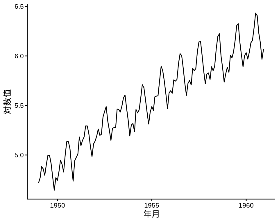
因此，下面基于对数尺度建模。首先考虑 RW1 随机游走模型，而后考虑季节性。RW1 模型意味着取对数、一阶差分后序列平稳高斯过程，序列值服从高斯分布。下面设置似然函数的高斯先验 $N (1, 0.2)$ ，目的是防止过拟合。

library(INLA)
inla.setOption(short.summary = TRUE)
air_passengers_df <- data.frame(
  y = as.vector(AirPassengers),
  year = as.factor(rep(1949:1960, each = 12)),
  month = as.factor(rep(1:12, times = 12)),
  ID = 1:length(AirPassengers)
)
mod_inla_rw1 <- inla(
  formula = log(y) ~ year + f(ID, model = "rw1"),
  family = "gaussian", data = air_passengers_df,
  control.family = list(hyper = list(prec = list(param = c(1, 0.2)))),
  control.predictor = list(compute = TRUE)
)
summary(mod_inla_rw1)

#> Fixed effects:
#>              mean    sd 0.025quant 0.5quant 0.975quant  mode kld
#> (Intercept) 5.159 0.252      4.666    5.158      5.657 5.158   0
#> year1950    0.050 0.134     -0.215    0.050      0.313 0.050   0
#> year1951    0.174 0.190     -0.201    0.174      0.546 0.174   0
#> year1952    0.262 0.233     -0.198    0.262      0.717 0.262   0
#> year1953    0.330 0.269     -0.201    0.331      0.857 0.331   0
#> year1954    0.357 0.301     -0.236    0.358      0.945 0.358   0
#> year1955    0.442 0.329     -0.208    0.443      1.086 0.443   0
#> year1956    0.510 0.356     -0.193    0.511      1.206 0.511   0
#> year1957    0.567 0.381     -0.184    0.568      1.311 0.568   0
#> year1958    0.576 0.403     -0.220    0.577      1.365 0.577   0
#> year1959    0.647 0.425     -0.191    0.648      1.478 0.648   0
#> year1960    0.683 0.445     -0.195    0.684      1.555 0.684   0
#> 
#> Model hyperparameters:
#>                                           mean    sd 0.025quant 0.5quant
#> Precision for the Gaussian observations 101.38 18.14      69.78    99.99
#> Precision for ID                        155.14 40.69      92.69   149.32
#>                                         0.975quant   mode
#> Precision for the Gaussian observations     140.94  97.59
#> Precision for ID                            251.66 137.49
#> 
#>  is computed

这里，将年份作为因子型变量，从输出结果可以看出，以1949年作为参照，回归系数的后验均值在逐年变大，这符合 AirPassengers 时序图呈现的趋势。

存在周期性的波动规律，考虑季节性

mod_inla_sea <- inla(
  formula = log(y) ~ year + f(ID, model = "seasonal", season.length = 12),
  family = "gaussian", data = air_passengers_df,
  control.family = list(hyper = list(prec = list(param = c(1, 0.2)))),
  control.predictor = list(compute = TRUE)
)
summary(mod_inla_sea)

#> Fixed effects:
#>              mean    sd 0.025quant 0.5quant 0.975quant  mode kld
#> (Intercept) 4.836 0.020      4.797    4.836      4.875 4.836   0
#> year1950    0.095 0.028      0.039    0.095      0.150 0.095   0
#> year1951    0.295 0.028      0.240    0.295      0.351 0.295   0
#> year1952    0.441 0.028      0.386    0.441      0.496 0.441   0
#> year1953    0.573 0.028      0.517    0.573      0.628 0.573   0
#> year1954    0.630 0.028      0.575    0.630      0.686 0.630   0
#> year1955    0.803 0.028      0.748    0.803      0.859 0.803   0
#> year1956    0.948 0.028      0.893    0.948      1.004 0.948   0
#> year1957    1.062 0.028      1.007    1.062      1.118 1.062   0
#> year1958    1.094 0.028      1.039    1.094      1.150 1.094   0
#> year1959    1.212 0.028      1.157    1.212      1.268 1.212   0
#> year1960    1.318 0.028      1.263    1.318      1.373 1.318   0
#> 
#> Model hyperparameters:
#>                                             mean       sd 0.025quant 0.5quant
#> Precision for the Gaussian observations   213.02    27.47     163.43   211.49
#> Precision for ID                        42099.89 27567.43   10148.84 35355.31
#>                                         0.975quant     mode
#> Precision for the Gaussian observations     271.39   208.87
#> Precision for ID                         113641.07 24337.17
#> 
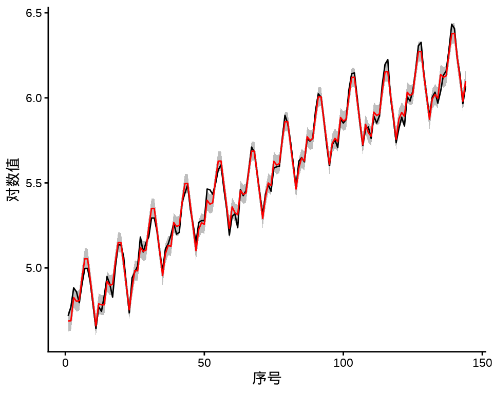
#>  is computed

最后，将两个模型的拟合结果展示出来，见下图，黑线表示原对数值，红线表示拟合值，灰色区域表示在置信水平 95% 下的区间。区间更短说明季节性模型更好。

mod_inla_rw1_fitted <- data.frame(
  ID = 1:length(AirPassengers),
  y = as.vector(log(AirPassengers)),
  mean = mod_inla_rw1$summary.fitted.values$mean,
  `0.025quant` = mod_inla_rw1$summary.fitted.values$`0.025quant`,
  `0.975quant` = mod_inla_rw1$summary.fitted.values$`0.975quant`,
  check.names = FALSE
)
mod_inla_sea_fitted <- data.frame(
  ID = 1:length(AirPassengers),
  y = as.vector(log(AirPassengers)),
  mean = mod_inla_sea$summary.fitted.values$mean,
  `0.025quant` = mod_inla_sea$summary.fitted.values$`0.025quant`,
  `0.975quant` = mod_inla_sea$summary.fitted.values$`0.975quant`,
  check.names = FALSE
)
ggplot(data = mod_inla_rw1_fitted, aes(ID)) +
  geom_ribbon(aes(ymin = `0.025quant`, ymax = `0.975quant`), fill = "gray") +
  geom_line(aes(y = y)) +
  geom_line(aes(y = mean), color = "red") +
  theme_classic() +
  labs(x = "序号", y = "对数值")
ggplot(data = mod_inla_sea_fitted, aes(ID)) +
  geom_ribbon(aes(ymin = `0.025quant`, ymax = `0.975quant`), fill = "gray") +
  geom_line(aes(y = y)) +
  geom_line(aes(y = mean), color = "red") +
  theme_classic() +
  labs(x = "序号", y = "对数值")

11.3 一些非参数模型

11.3.1 mgcv 包

mgcv 包 (S. N. Wood 2017) 是 R 软件内置的推荐组件，由 Simon Wood 开发和维护，历经多年，成熟稳定。函数 bam() 相比于函数 gam() 的优势是可以处理大规模的时间序列数据。对于时间序列数据预测，数万和百万级观测值都可以 (Simon N. Wood, Goude, 和 Shaw 2015)。

air_passengers_tbl <- data.frame(
  y = as.vector(AirPassengers),
  year = rep(1949:1960, each = 12),
  month = rep(1:12, times = 12)
)
mod1 <- gam(log(y) ~ s(year) + s(month, bs = "cr"),
  data = air_passengers_tbl, family = gaussian
)
summary(mod1)

#> 
#> Family: gaussian 
#> Link function: identity 
#> 
#> Formula:
#> log(y) ~ s(year) + s(month, bs = "cr")
#> 
#> Parametric coefficients:
#>             Estimate Std. Error t value Pr(>|t|)    
#> (Intercept) 5.542176   0.003456    1604   <2e-16 ***
#> ---
#> Signif. codes:  0 '***' 0.001 '**' 0.01 '*' 0.05 '.' 0.1 ' ' 1
#> 
#> Approximate significance of smooth terms:
#>            edf Ref.df      F p-value    
#> s(year)  7.947  8.712 1688.9  <2e-16 ***
#> s(month) 8.769  8.983  150.6  <2e-16 ***
#> ---
#> Signif. codes:  0 '***' 0.001 '**' 0.01 '*' 0.05 '.' 0.1 ' ' 1
#> 
#> R-sq.(adj) =  0.991   Deviance explained = 99.2%
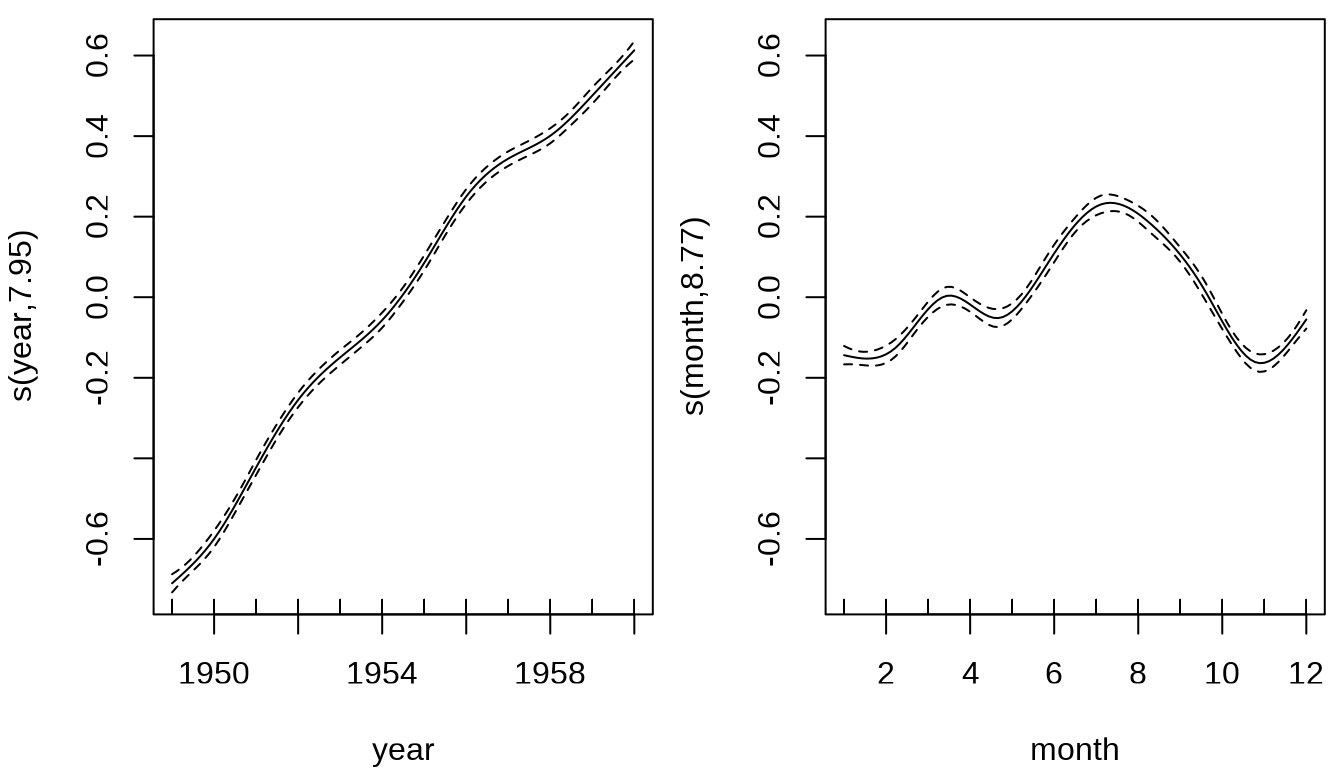
#> GCV = 0.0019614  Scale est. = 0.0017201  n = 144

观察年和月的趋势变化，逐年增长趋势基本是线性的，略有波动，逐月变化趋势比较复杂，不过，可以明显看出在 7-9 月是高峰期，11 月和1-3月是低谷期。

layout(matrix(1:2, nrow = 1))
plot(mod1, shade = TRUE)

将拟合效果绘制出来，见下图，整体上，捕捉到了趋势和周期，不过，存在欠拟合，年周期内波动幅度随时间有变化趋势，趋势和周期存在交互作用。

air_passengers_ts <- ts(exp(mod1$fitted.values), start = c(1949, 1), frequency = 12)
plot(AirPassengers)
lines(air_passengers_ts, col = "red")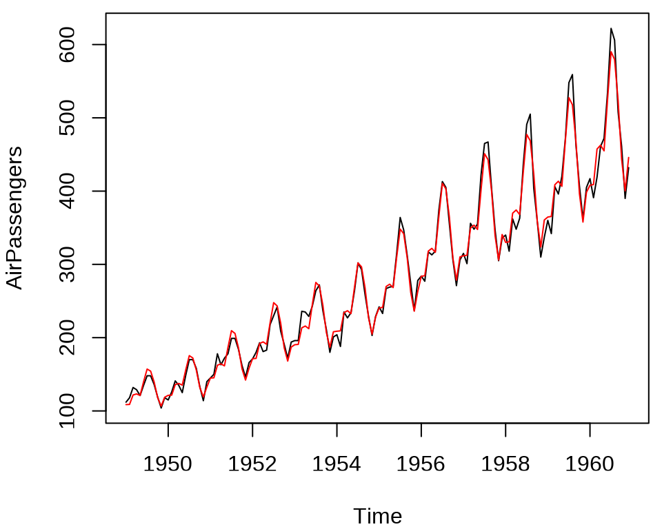

整体上，乘客数逐年呈线性增长，每年不同月份呈现波动，淡季和旺季出行的流量有很大差异，近年来，这种差异的波动在扩大。为了刻画这种情况，考虑年度趋势和月度波动的交互作用。

mod2 <- gam(log(y) ~ s(year, month), data = air_passengers_tbl, family = gaussian)
summary(mod2)

#> 
#> Family: gaussian 
#> Link function: identity 
#> 
#> Formula:
#> log(y) ~ s(year, month)
#> 
#> Parametric coefficients:
#>             Estimate Std. Error t value Pr(>|t|)    
#> (Intercept) 5.542176   0.004491    1234   <2e-16 ***
#> ---
#> Signif. codes:  0 '***' 0.001 '**' 0.01 '*' 0.05 '.' 0.1 ' ' 1
#> 
#> Approximate significance of smooth terms:
#>                 edf Ref.df     F p-value    
#> s(year,month) 26.94  28.74 329.2  <2e-16 ***
#> ---
#> Signif. codes:  0 '***' 0.001 '**' 0.01 '*' 0.05 '.' 0.1 ' ' 1
#> 
#> R-sq.(adj) =  0.985   Deviance explained = 98.8%
#> GCV = 0.003603  Scale est. = 0.0029039  n = 144

可以看到，调整的 $R^{2}$ 明显增加，拟合效果更好，各年各月份的乘客数变化，见下图。

op <- par(mar = c(4, 4, 2, 0))
plot(mod2)
on.exit(par(op), add = TRUE)

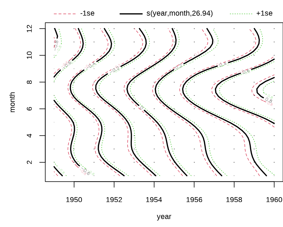
上图是轮廓图，下面用透视图展示趋势拟合的效果。

op <- par(mar = c(0, 1.5, 0, 0))
vis.gam(mod2, theta = -35, phi = 20, ticktype = "detailed", expand = .65, zlab = "")
on.exit(par(op), add = TRUE)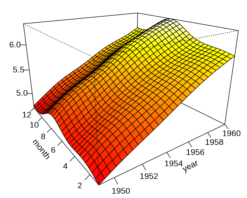

最后，在原始数据的基础上，添加拟合数据，得到如下拟合趋势图，与前面的拟合图比较，可以看出效果提升很明显。

air_passengers_ts <- ts(exp(mod2$fitted.values), start = c(1949, 1), frequency = 12)
plot(AirPassengers)
lines(air_passengers_ts, col = "red")

11.3.2 nnet 包

前面介绍的模型都具有非常强的可解释性，比如各个参数对模型的作用。对于复杂的时间序列数据，比较适合用复杂的模型来拟合，看重模型的泛化能力，而不那么关注模型的机理。

多层感知机是一种全连接层的前馈神经网络。nnet 包的函数 nnet() 实现了单隐藏层的简单前馈神经网络，可用于时间序列预测，也可用于分类数据的预测。作为对比的基础，下面先用 nnet 包训练和预测数据。

# 准备数据
air_passengers <- as.matrix(embed(AirPassengers, 4))
colnames(air_passengers) <- c("y", "x3", "x2", "x1")
data_size <- nrow(air_passengers)
# 拆分数据集
train_size <- floor(data_size * 0.67)
train_data <- air_passengers[1:train_size, ]
test_data <- air_passengers[-(1:train_size), ]

# 随机数种子对结果的影响非常大 试试 set.seed(20232023) 
set.seed(20222022) 
# 单隐藏层 8 个神经元
mod_nnet <- nnet::nnet(
  y ~ x1 + x2 + x3,
  data = air_passengers, # 数据集
  subset = 1:train_size, # 训练数据的指标向量
  linout = TRUE, size = 4, rang = 0.1,
  decay = 5e-4, maxit = 400, trace = FALSE
)
# 预测
train_pred <- predict(mod_nnet, newdata = air_passengers[1:train_size,], type = "raw")
# 训练集 RMSE
sqrt(mean((air_passengers[1:train_size, "y"] - train_pred )^2))

#> [1] 21.59392

# 预测
test_pred <- predict(mod_nnet, newdata = air_passengers[-(1:train_size),], type = "raw")
# 测试集 RMSE
sqrt(mean((air_passengers[-(1:train_size), "y"] - test_pred)^2))

#> [1] 53.79107

下面将原观测序列，训练集和测试集上的预测序列放在一张图上展示。图中，红色曲线表示训练集上的预测结果，绿色曲线为测试集上预测结果。

train_pred_ts <- ts(data = train_pred, start = c(1949, 3), frequency = 12)
test_pred_ts <- ts(data = test_pred, start = c(1957, 1), frequency = 12)
plot(AirPassengers)
lines(train_pred_ts, col = "red")
lines(test_pred_ts, col = "green")

由图可知，在测试集上，随着时间拉长，预测越来越不准。

11.3.3 keras3 包

keras3 包通过 reticulate 包引入 Keras 3 框架，这个框架支持 TensorFlow 和 PyTorch 等多个后端，目前，keras3 包通过 tensorflow 包仅支持 TensorFlow 后端。

下面使用 keras3 包构造多层感知机训练数据和预测。

library(keras3)
set_random_seed(20222022)
# 模型结构
mod_mlp <- keras_model_sequential(shape = c(3)) |> 
  layer_dense(units = 12, activation = "relu") |> 
  layer_dense(units = 8, activation = "relu") |> 
  layer_dense(units = 1)
# 训练目标
compile(mod_mlp,
  loss = "mse", # 损失函数
  optimizer = "adam", # 优化器
  metrics = "mae" # 监控度量
)
# 模型概览
summary(mod_mlp)

#> Model: "sequential"
#> ┏━━━━━━━━━━━━━━━━━━━━━━━━━━━━━━━━━━━┳━━━━━━━━━━━━━━━━━━━━━━━━━━┳━━━━━━━━━━━━━━━┓
#> ┃ Layer (type)                      ┃ Output Shape             ┃       Param # ┃
#> ┡━━━━━━━━━━━━━━━━━━━━━━━━━━━━━━━━━━━╇━━━━━━━━━━━━━━━━━━━━━━━━━━╇━━━━━━━━━━━━━━━┩
#> │ dense (Dense)                     │ (None, 12)               │            48 │
#> ├───────────────────────────────────┼──────────────────────────┼───────────────┤
#> │ dense_1 (Dense)                   │ (None, 8)                │           104 │
#> ├───────────────────────────────────┼──────────────────────────┼───────────────┤
#> │ dense_2 (Dense)                   │ (None, 1)                │             9 │
#> └───────────────────────────────────┴──────────────────────────┴───────────────┘
#>  Total params: 161 (644.00 B)
#>  Trainable params: 161 (644.00 B)
#>  Non-trainable params: 0 (0.00 B)

输入层为 3 个节点，中间两个隐藏层，第一层为 12 个节点，第二层为 8 个节点，全连接网络，最后输出为一层单节点，意味着单个输出。每一层都有节点和权重，参数总数为 161。

# 拟合模型
fit(mod_mlp,
  x = train_data[, c("x1", "x2", "x3")],
  y = train_data[, "y"],
  epochs = 200,
  batch_size = 10, # 每次更新梯度所用的样本量
  validation_split = 0.2, # 从训练数据中拆分一部分用作验证集
  verbose = 0 # 不显示训练进度
)
# 将测试数据代入模型，计算损失函数和监控度量
evaluate(mod_mlp, test_data[, c("x1", "x2", "x3")], test_data[, "y"])

#> 2/2 - 0s - 12ms/step - loss: 2580.7053 - mae: 41.8020

#> $loss
#> [1] 2580.705
#> 
#> $mae
#> [1] 41.80202

# 测试集上的预测
mlp_test_pred <- predict(mod_mlp, test_data[, c("x1", "x2", "x3")])

#> 2/2 - 0s - 28ms/step

mlp_train_pred <- predict(mod_mlp, train_data[, c("x1", "x2", "x3")])

#> 3/3 - 0s - 7ms/step

sqrt(mean((test_data[, "y"] - mlp_test_pred)^2)) # 计算均方根误差

#> [1] 50.80064

从 RMSE 来看，MLP（多层感知机）预测效果比单层感知机稍好些，可网络复杂度是增加很多的。

mlp_train_pred_ts <- ts(data = mlp_train_pred, start = c(1949, 3), frequency = 12)
mlp_test_pred_ts <- ts(data = mlp_test_pred, start = c(1957, 1), frequency = 12)
plot(AirPassengers)
lines(mlp_train_pred_ts, col = "red")
lines(mlp_test_pred_ts, col = "green")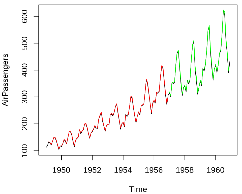

下面用 LSTM （长短期记忆）神经网络来训练时间序列数据，预测未来一周的趋势。输出不再是一天（单点输出），而是 7 天的预测值（多点输出）。参考 tensorflow 包的官网中 RNN 递归神经网络的介绍。

11.4 习题

基于 R 软件内置的数据集 sunspots 和 sunspot.month 比较 INLA 和 mgcv 框架的预测效果。

代码

sunspots_tbl <- broom::tidy(sunspots)
sunspots_month_tbl <- broom::tidy(sunspot.month)
ggplot() +
  geom_line(data = sunspots_month_tbl, aes(x = index, y = value), color = "red") +
  geom_line(data = sunspots_tbl, aes(x = index, y = value)) +
  theme_bw() +
  labs(x = "年月", y = "数量")

图中黑线和红线分别表示 1749-1983 年、1984-2014 年每月太阳黑子数量。