12 点模式数据分析
本章以斐济地震数据集 quakes 为例介绍空间点模式数据的操作、探索和分析。
spatstat 是一个伞包,囊括 8 个子包,构成一套完整的空间点模式分析工具。
- spatstat.utils 基础的辅助分析函数
- spatstat.data 点模式分析用到的示例数据集
- spatstat.sparse 稀疏数组
- spatstat.geom 空间数据类和几何操作
- spatstat.random 生成空间随机模式
- spatstat.explore 空间数据的探索分析
- spatstat.model 空间数据的参数建模和推理
- spatstat.linnet 线性网络上的空间分析
sf 包是一个专门用于空间矢量数据操作的 R 包。ggplot2 包提供的几何图层函数 geom_sf() 和坐标参考系图层函数 coord_sf() 支持可视化空间点模式数据。
12.1 数据操作
12.1.1 类型转化
先对斐济地震数据 quakes 数据集做一些数据类型转化,从 data.frame 转 Simple feature 对象。
#> Simple feature collection with 1000 features and 3 fields
#> Geometry type: POINT
#> Dimension:     XY
#> Bounding box:  xmin: 165.67 ymin: -38.59 xmax: 188.13 ymax: -10.72
#> Geodetic CRS:  WGS 84
#> First 10 features:
#>    depth mag stations              geometry
#> 1    562 4.8       41 POINT (181.62 -20.42)
#> 2    650 4.2       15 POINT (181.03 -20.62)
#> 3     42 5.4       43     POINT (184.1 -26)
#> 4    626 4.1       19 POINT (181.66 -17.97)
#> 5    649 4.0       11 POINT (181.96 -20.42)
#> 6    195 4.0       12 POINT (184.31 -19.68)
#> 7     82 4.8       43   POINT (166.1 -11.7)
#> 8    194 4.4       15 POINT (181.93 -28.11)
#> 9    211 4.7       35 POINT (181.74 -28.74)
#> 10   622 4.3       19 POINT (179.59 -17.47)
12.1.2 坐标转化
如果知道两个投影坐标系的 EPSG 代码,输入坐标就可以完成转化。如将坐标系 EPSG:4326 下的坐标 \((2,49)\) 投影到另一个坐标系 EPSG:3857 。
#> Geometry set for 1 feature
#> Geometry type: POINT
#> Dimension:     XY
#> Bounding box:  xmin: 222639 ymin: 6274861 xmax: 222639 ymax: 6274861
#> Projected CRS: WGS 84 / Pseudo-Mercator
#> POINT (222639 6274861)| 名称 | EPSG | 赤道半径 | 半轴 | 发明者 |
|---|---|---|---|---|
| GRS80 | 3857 | a=6378137.0 | rf=298.257222101 | GRS 1980(IUGG, 1980) |
| WGS84 | 4326 | a=6378137.0 | rf=298.257223563 | WGS 84 |
函数 st_crs() 查看坐标参考系的信息,比如 EPSG 代码为 4326 对应的坐标参考系统信息。我们也可以通过网站查询 EPSG 代码对应的坐标参考系统的详细介绍。
#> Coordinate Reference System:
#>   User input: EPSG:4326
#>   wkt:
#> GEOGCRS["WGS 84",
#>     ENSEMBLE["World Geodetic System 1984 ensemble",
#>         MEMBER["World Geodetic System 1984 (Transit)"],
#>         MEMBER["World Geodetic System 1984 (G730)"],
#>         MEMBER["World Geodetic System 1984 (G873)"],
#>         MEMBER["World Geodetic System 1984 (G1150)"],
#>         MEMBER["World Geodetic System 1984 (G1674)"],
#>         MEMBER["World Geodetic System 1984 (G1762)"],
#>         MEMBER["World Geodetic System 1984 (G2139)"],
#>         ELLIPSOID["WGS 84",6378137,298.257223563,
#>             LENGTHUNIT["metre",1]],
#>         ENSEMBLEACCURACY[2.0]],
#>     PRIMEM["Greenwich",0,
#>         ANGLEUNIT["degree",0.0174532925199433]],
#>     CS[ellipsoidal,2],
#>         AXIS["geodetic latitude (Lat)",north,
#>             ORDER[1],
#>             ANGLEUNIT["degree",0.0174532925199433]],
#>         AXIS["geodetic longitude (Lon)",east,
#>             ORDER[2],
#>             ANGLEUNIT["degree",0.0174532925199433]],
#>     USAGE[
#>         SCOPE["Horizontal component of 3D system."],
#>         AREA["World."],
#>         BBOX[-90,-180,90,180]],
#>     ID["EPSG",4326]]
地球看作一个椭球体 ELLIPSOID,长半轴 6378137 米,短半轴 298.257223563 米,椭圆形的两个轴,纬度单位 0.0174532925199433, 经度单位 0.0174532925199433 。
地球是一个不规则的球体,不同的坐标参考系对地球的抽象简化不同,会体现在坐标原点、长半轴、短半轴等属性上。为了方便在平面上展示地理信息,需要将地球表面投影到平面上,墨卡托投影是其中非常重要的一种投影方式,墨卡托投影的详细介绍见 PROJ 网站 。WGS 84 / Pseudo-Mercator 投影主要用于网页上的地理可视化,UTM 是 Universal Transverse Mercator 的缩写。360 度对应全球 60 个时区,每个时区横跨 6 经度。
st_transform(
  x = st_sfc(st_point(x = c(2, 49)), crs = 4326),
  crs = st_crs("+proj=utm +zone=32 +ellps=GRS80")
)
#> Geometry set for 1 feature
#> Geometry type: POINT
#> Dimension: XY
#> Bounding box: xmin: -11818.95 ymin: 5451107 xmax: -11818.95 ymax: 5451107
#> Projected CRS: +proj=utm +zone=32 +ellps=GRS80#> POINT (-11818.95 5451107)快速简单绘图,可采用图层 geom_sf(),它相当于统计图层 stat_sf() 和坐标映射图层 coord_sf() 的叠加,geom_sf() 支持点、线和多边形等数据数据对象,可以混合叠加。 coord_sf() 有几个重要的参数:
crs:在绘图前将各个geom_sf()图层中的数据映射到该坐标参考系。default_crs:将非 sf 图层(没有携带 CRS 信息)的数据映射到该坐标参考系,默认使用crs参数的值,常用设置default_crs = sf::st_crs(4326)将非 sf 图层中的横纵坐标转化为经纬度,采用 World Geodetic System 1984 (WGS84)。datum:经纬网线的坐标参考系,默认值sf::st_crs(4326)。
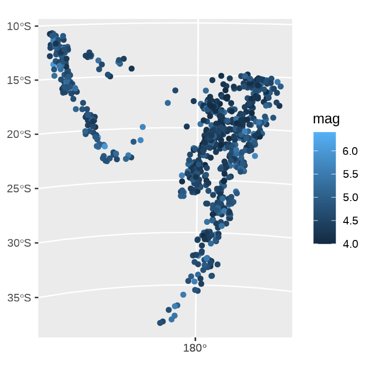
下图的右子图将 quakes_sf 数据集投影到坐标参考系统EPSG:3460。
library(ggplot2)
ggplot() +
  geom_sf(data = quakes_sf, aes(color = mag))
ggplot() +
  geom_sf(data = quakes_sf, aes(color = mag)) +
  coord_sf(crs = 3460)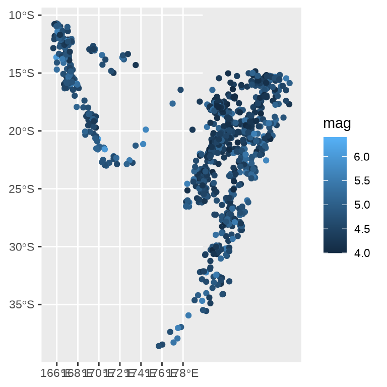
数据集 quakes_sf 已经准备了坐标参考系统,此时,coord_sf() 就会采用数据集相应的坐标参考系统,即 sf::st_crs(4326)。上图的左子图相当于:
12.1.3 凸包操作
# 绘制点及其包络
plot(st_geometry(quakes_sf))
# 添加凸包曲线
plot(quakes_sfp_hull, add = TRUE)
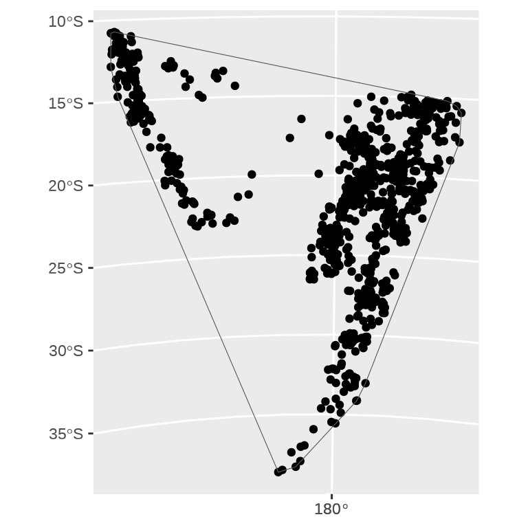
ggplot() +
geom_sf(data = quakes_sf) +
geom_sf(data = quakes_sfp_hull, fill = NA) +
coord_sf(crs = 3460, xlim = c(569061, 3008322), ylim = c(1603260, 4665206))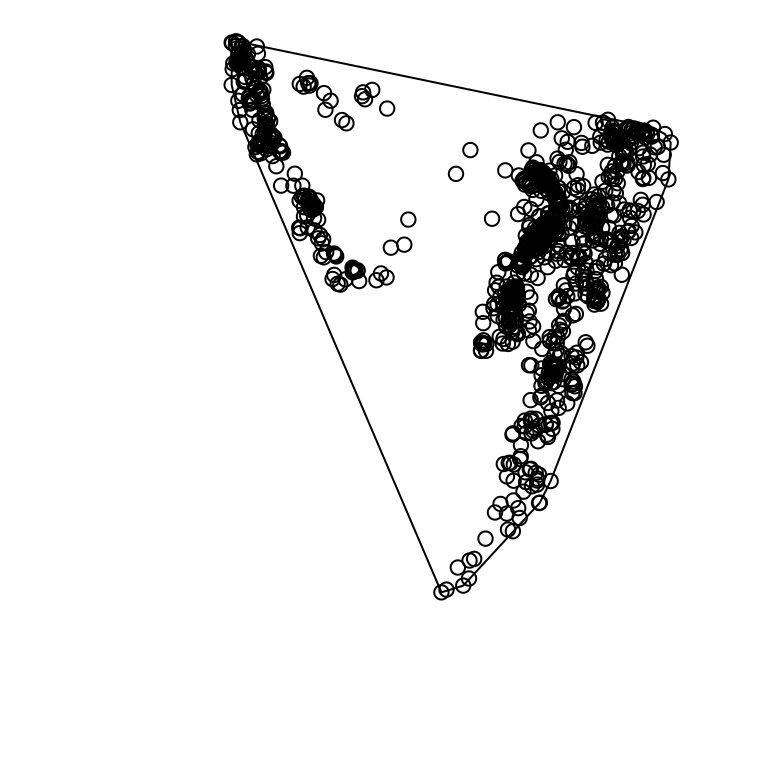
12.2 数据探索
12.2.1 核密度估计
给定边界内的核密度估计与绘制热力图
# spatial point pattern ppp 类型
quakes_ppp <- spatstat.geom::as.ppp(st_geometry(quakes_sf))
# 限制散点在给定的窗口边界内平滑
spatstat.geom::Window(quakes_ppp) <- spatstat.geom::as.owin(quakes_sfp_hull)
#> Warning: point-in-polygon test had difficulty with 1 point (total score not 0
#> or 1)# quakes_ppp <- spatstat.geom::as.ppp(st_geometry(quakes_sf), W = spatstat.geom::as.owin(quakes_sfp_hull))
# 密度估计
density_spatstat <- spatstat.explore::density.ppp(quakes_ppp, dimyx = 256)
# 转化为 stars 对象 栅格数据
density_stars <- stars::st_as_stars(density_spatstat)
# 设置坐标参考系
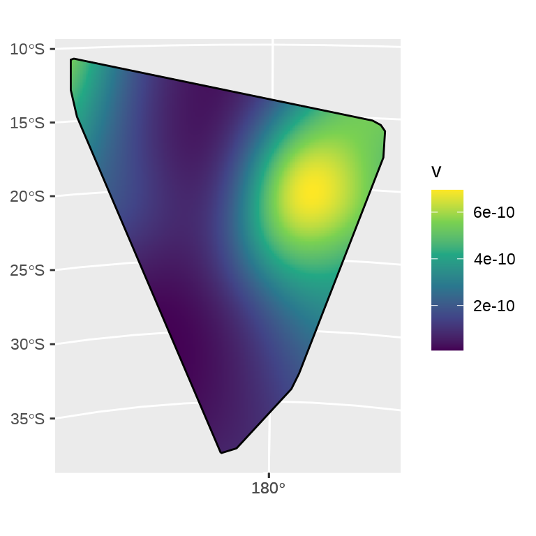
density_sf <- st_set_crs(st_as_sf(density_stars), 3460)12.2.2 绘制热力图
ggplot() +
geom_sf(data = density_sf, aes(fill = v), col = NA) +
scale_fill_viridis_c() +
geom_sf(data = st_boundary(quakes_sfp_hull))
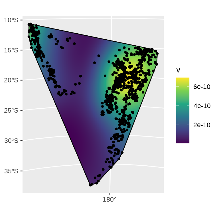
ggplot() +
geom_sf(data = density_sf, aes(fill = v), col = NA) +
scale_fill_viridis_c() +
geom_sf(data = st_boundary(quakes_sfp_hull)) +
geom_sf(data = quakes_sf, size = 1, col = "black")