第 17 章 利用文本挖掘技术分析文献摘要
library(tidyverse)
library(here)
library(fs)
library(purrr)
library(tidytext)
library(widyr)
library(tidygraph)
library(ggraph)本章基于R语言文本挖掘技术,分析文献摘要。具体做法是,利用R语言tidyverse、tidytext、widyr、tidygraph、ggraph等宏包分析我校文献(Web of Science)摘要的文本信息。6
17.1 数据导入
为了研究的可重复性,我列出了数据获取步骤: - 打开https://www.webofknowledge.com/,进入核心合集 - 输入学校全名:比如 Sichuan Normal University - 选择“机构扩展”检索 - 选择时间范围:“2009-2018年” - 选择“SCI/SSCI/A&HCI” - 点击检索 - 文档类型精炼:”Article + Review “ - 一次显示最多 50 条,一次下载最多 500 条 - 选择“其他类型下载” + “全记录与引用的参考文献” + “win UTF” - 依此下载保存
我们共获取了 1988 条文献题录数据。
read_plus <- function(flnm) {
read_tsv(flnm, quote = "", col_names = TRUE) %>%
#or
#read_delim(flnm, delim="\t" , quote = "", col_names = TRUE) %>%
#select(AU, AF, SO, DE, C1, RP, FU, CR, TC, SN, PY, UT) %>%
select(AB, SN, UT) #%>%
# mutate(University = flnm %>% # 加入了学校名
# str_split("/", 7, simplify = TRUE) %>%
# .[, 6] %>%
# str_sub(start = 4)
# )
}tbl <- here("data", "newdata") %>%
dir_ls(regexp = "*.txt", recursive = TRUE) %>%
map_dfr(~read_plus(.))
tblesi_plus_cas_IF_set <- read_rds(here("data", "esiJournalsList", "esi_plus_cas_IF_set.rds"))
complete_set <- tbl %>%
left_join(esi_plus_cas_IF_set, by = c("SN" = "ISSN") ) %>%
select(category = Category_ESI_cn, abstract = AB, pubs = UT) #%>%
# rename(ISSN = SN) %>% 17.2 数据规整
complete_set数据整理和文本分词
text_df <- complete_set %>%
filter(!is.na(abstract)) %>%
unnest_tokens(output = grams, input = abstract, token = "ngrams", n = 2)
text_df过滤无用词汇
text_filted <- text_df %>%
separate(grams, into = c("word1", "word2"), sep = " ") %>%
filter(!word1 %in% stop_words$word) %>%
filter(!word2 %in% stop_words$word)
text_filted text_unite <- text_filted %>%
unite(grams, word1, word2, sep = " ")
text_unite17.3 计算tf_idf
text_tf_idf <- text_unite %>%
count(pubs, grams) %>%
bind_tf_idf(pubs, grams, n) %>%
arrange(desc(tf_idf))
text_tf_idftext_tf_idf %>% group_by(pubs) %>%
filter(max(tf_idf) > 9.1) %>%
#dplyr::distinct(pubs)
ggplot(aes(x = fct_reorder(grams, tf_idf), y = tf_idf, fill = pubs)) +
geom_col(show.legend = FALSE) +
coord_flip() +
facet_wrap(vars(pubs), ncol = 2, scales = "free")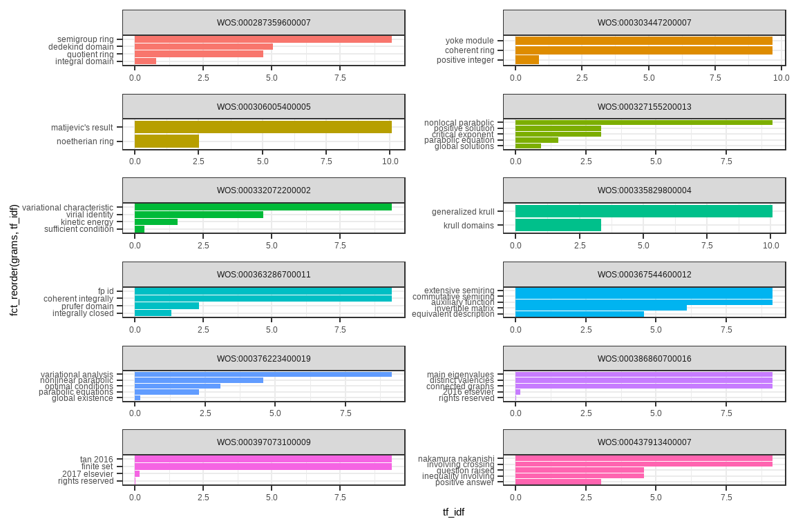
17.4 文本相似性
\[ \text{similarity} = \cos ( \theta ) = \frac { \mathbf { A } \cdot \mathbf { B } } { \| \mathbf { A } \| \| \mathbf { B } \| } = \frac { \sum _ { i = 1 } ^ { n } A _ { i } B _ { i } } { \sqrt { \sum _ { i = 1 } ^ { n } A _ { i } ^ { 2 } } \sqrt { \sum _ { i = 1 } ^ { n } B _ { i } ^ { 2 } } } \]
text_tf_idf %>%
pairwise_similarity(pubs, grams, tf_idf, upper = FALSE, sort = TRUE)17.5 关联词汇
前面我们计算了过滤词汇text_filted,我们现在研究这些词汇之间的关联
text_count <- text_filted %>%
count(category, word1, word2, sort = TRUE) %>%
select(word1, word2, n, category) %>%
arrange(category)
text_counttext_count %>%
filter(n > 20) %>%
as_tbl_graph() ## # A tbl_graph: 124 nodes and 94 edges
## #
## # A directed multigraph with 46 components
## #
## # Node Data: 124 x 1 (active)
## name
## <chr>
## 1 piezoelectric
## 2 rights
## 3 lead
## 4 elsevier
## 5 sintering
## 6 phase
## # ... with 118 more rows
## #
## # Edge Data: 94 x 4
## from to n category
## <int> <int> <int> <chr>
## 1 1 74 65 材料科学
## 2 2 75 58 材料科学
## 3 3 52 45 材料科学
## # ... with 91 more rowstext_count %>%
filter(n > 20) %>%
as_tbl_graph() %>%
ggraph(layout = "fr") +
geom_node_point() +
geom_edge_link(aes(color = category, edge_width = n)) +
geom_node_text(aes(label = name), repel = TRUE) +
#facet_wrap(vars(category), ncol = 3, scales = "free")
facet_edges(vars(category), ncol = 3, scales = "free")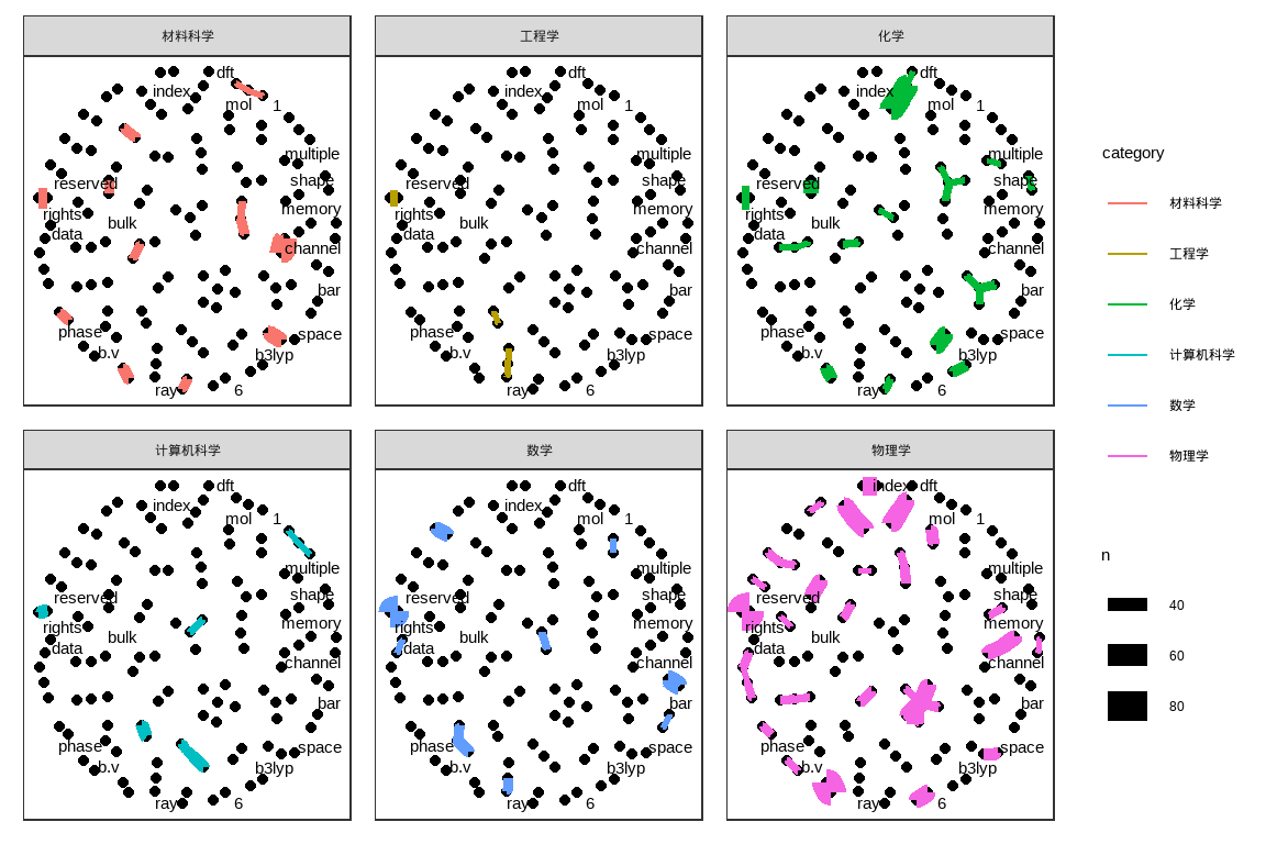
17.6 下一步工作
- 数据量很多,需要精炼,从而提前有用的关键信息
- 还没想好