Chapter 11 Vector Calculus
- MML, chapter 5
11.1 理論
\[ {\bf f(\theta)=}\begin{bmatrix}f_{1}({\bf \theta})\\ \vdots\\ f_{m}({\bf \theta}) \end{bmatrix}\in\mathbb{R}^{m\times1} \]
- \(m\)個函數
\[ {\bf f(\theta)}=\begin{bmatrix} a1*\theta_1+a2*\theta_2+a3*\theta_3\\ b1*\theta_1^2+b2*\theta_2^3 \end{bmatrix} \]
numpy有一系列的polynomial routines
擴充前述的函數,允許input x可以有任意的維度,函數也可以有任意的維度及不同多向式。
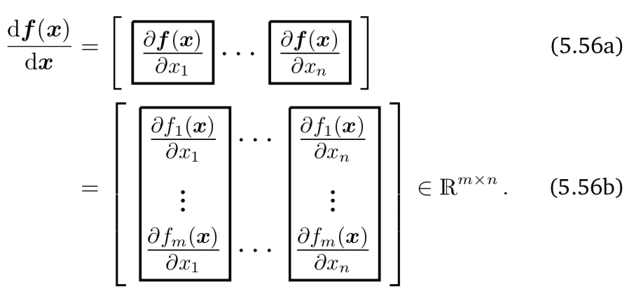
\[ \frac{\partial{\bf f(\theta)}}{\partial \theta_{i}}{\bf =}\begin{bmatrix}\frac{\partial f_{1}({\bf \theta})}{\partial \theta_{i}}\\ \vdots\\ \frac{\partial f_{m}({\bf \theta})}{\partial \theta_{i}} \end{bmatrix}\in\mathbb{R}^{m\times1} \]


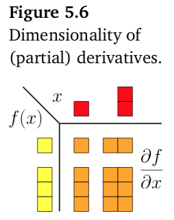
Figure 11.1: 向量函數維度
11.1.1 Jacobian
The collection of all first-order partial deriva- tives of a vector-valued function is called the Jacobian.
11.2 Gradient Descent
\[\min_{\theta} f(\theta)\]
\(\nabla_{\theta}f(\theta)\) gives that direction that can increases f value. To decrease value, we need to go \(-\nabla_{\theta}f(\theta)\) direction。
Only direction, but how long? \(-\gamma \nabla_{\theta}f(\theta)\)
11.2.1 Vanilla gradient descent
\[\theta_{i+1}=\theta_{i}-\gamma \nabla_{\theta}f(\theta_i)\]
11.2.2 Adaptive gradient descent
\[\theta_{i+1}=\theta_{i}-\gamma_i \nabla_{\theta}f(\theta_i)\]
- \(\gamma_i\) is called the learning rate.
- When the function value increases after a gradient step, the step-size was too large. Undo the step and decrease the step-size.
- When the function value decreases the step could have been larger. Try to increase the step-size.
- When the function value increases after a gradient step, the step-size was too large. Undo the step and decrease the step-size.
11.2.3 Gradient Descent With Momentum
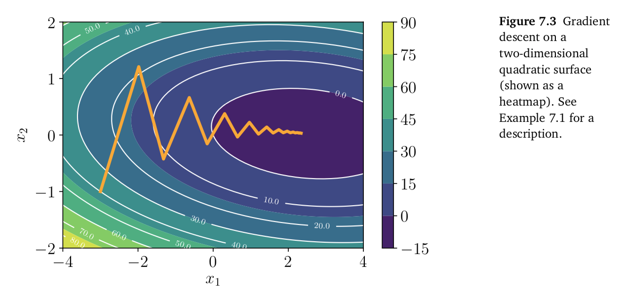
As illustrated in Figure 7.3, the convergence of gradient descent may be very slow if the curvature of the optimization surface is such that there are regions that are poorly scaled.

\[\theta_{i+1}=\theta_{i}-\gamma_i \nabla_{\theta}f(\theta_i)+ \alpha \Delta \theta_i\]
11.2.4 Stochastic Gradient Descent
\[ f(\theta)=\sum_{n=1}^N f(\theta | \bf x_n)\]
Vanilla gradient descent:
\[ \begin{eqnarray} \theta_{i+1} &=& \theta_{i}-\gamma \nabla_{\theta}f(\theta_i)\\ &=& \theta_{i}-\gamma \sum_{n=1}^N \nabla_{\theta}f(\theta_i|\bf x_n) \end{eqnarray}\]
N can be huge.
Randomly draw a mini-batch \(B_i\) from training data. And consider the following loss function instead:
\[f_{B_i}(\theta) =\sum_{\bf x_n\in B_{i}}f(\theta|\bf x_n)\]
Mini-batch Stochastic Gradient Descet:
\[\theta_{i+1}=\theta_{i}-\gamma \sum_{\bf x_n\in B_{i}} \nabla_{\theta}f(\theta_i|\bf x_n)\]
Batch Gradient Descent. Batch Size = Size of Training Set
Stochastic Gradient Descent. Batch Size = 1
Mini-Batch Gradient Descent. 1 < Batch Size < Size of Training Set
We will divided training set into several mini batches. And use each through several iterations.
- Epochs