Chapter 7 Probability and Distribution
- Mathematics for Machine Learning (MML), chapter 6.
7.1 Probability space
由\((\Omega,\mathcal{A},P)\)三元素構成:
The sample space Ω
The sample space is the set of all possible outcomes (\(\omega\)’s) of the experiment, usually denoted by Ω. For example, two successive coin tosses have a sample space of \({hh, tt, ht, th}\), where “h” denotes “heads” and “t” denotes “tails”.
\[\Omega=\{\omega_1,\omega_2,\dots,\omega_n\}\]
The experiment: tossing twice
Set of all possible outcomes, 稱\(\Omega_{2}\)為二次擲幣實驗下的sample space,則:
\[\Omega_{2}=\{("h","h"),("h","t"),("t","h"),("t","t")\}\]
\(\omega\)’s 指得是?
Python: Sample space
The first element represents the outcome of first toss, and the second element represents the second toss. Using tuple, the immutability means that elements inside the tuple are not exchangable.
7.1.1 The event space \(\mathcal{A}\)
The event space is the space of potential results of the experiment. A subset A of the sample space Ω is in the event space \(\mathcal{A}\) if at the end of the experiment we can observe whether a particular outcome ω ∈ Ω is in A. The event space A is obtained by considering the collection of subsets of Ω.
The collection of subsets of \(\Omega_{2}\):
- 任何可以成為\(\Omega_{2}\) subset的set都屬於event space一員。
The relational symbol for subset is: \(\subseteq\)
# subset
Omega_2

{('t','h')}.issubset(Omega_2)
{('t', 'h'), ('h', 'h')}.issubset(Omega_2)
set([]).issubset(Omega_2) # 空集合 (empty set/ null set)
Omega_2.issubset(Omega_2) # sample space itself- Empty set and the sample space must be part of the event space.
原則上set只能放immutable (unhashable)成員。
- 直覺,若mutable,有可能改變內容使set出現重複元素。
- frozenset是immutable的set。
Python: Event space
The event space \(\mathcal{A}\) is denoted as A_big here:
import itertools

maxN=len(Omega_2)
for outcomeNumber in range(1,maxN):
    for ix in itertools.combinations(Omega_2, outcomeNumber): # (1)
        A_big.add(frozenset(ix))

print(A_big)- (1):
itertools.combinations(Omega_2, outcomeNumber), all possible sets ofdistinct elements from Omega_2.
You probably notice that the combinations add to the set do not seem to follow any order. This is because in Python:
list and tuple are sequential.
set and dictionary are not sequential, which element will pop up for next iteration will depend on computer memory mangement.
How many events are in this event space?
Verify that every event in A_big is a subset of Omega_2.
7.1.2 The probability P
With each event A ∈ \(\mathcal{A}\), we associate a number P (A) that measures the probability or degree of belief that the event will occur. P (A) is called the probability of A.
We need a mapping P: \[A\stackrel{P}{\longrightarrow}[0,1],\mbox{ for all }A \in \mathcal{A},\] and P conforms with probability axioms.
Probability axioms ensure that \[P(A)=\sum_{\omega\in A} P(\omega).\] Therefore, once we define \(P(\omega)\) for all outcomes \(\omega\) in sample space \(\Omega\), \(P(A)\) is obtained.
Python: Probability of basic outcomes
import pandas as pd

Pt=0.5
Omega_2_a=np.array(list(Omega_2))
P_omega=Pt**(Omega_2_a[:,0]=='t')*(1-Pt)**(1-(Omega_2_a[:,0]=='t'))*Pt**(Omega_2_a[:,1]=='t')*(1-Pt)**(1-(Omega_2_a[:,1]=='t')) # [1]
P_omega=pd.Series(P_omega, index=Omega_2_a)
print(P_omega)
[1] Each \(\omega\) consists of two coin-toss outcomes, say \((t_1,t_2)\) where \(t_j\in \{"h","t"\}\). Therefore,
\[ \begin{eqnarray} P(\omega)&=&P(t_1,t_2)\\ &=& P(t_1="t")^{I(t_1=="t")}P(t_1="h")^{I(t_1=="h")}\times\\ & & P(t_2="t")^{I(t_2=="t")}P(t_2="h")^{I(t_2=="h")}, \end{eqnarray} \] given that \(P(t="h")=1-P(t="t")\) and \(I(.)\) is an indicator function producing boolean result.
There are two ways to define mapping:
dictionary with keys of every event and values of its corresponding probability.
function with event space as its domain and probability as its target value.
Python: Probability function
Find the probability of event_test from P_omega.
def P(A, Pt=0.5):
    Omega_2_a=np.array(list(Omega_2))
    P_omega=Pt**(Omega_2_a[:,0]=='t')*(1-Pt)**(1-(Omega_2_a[:,0]=='t'))*Pt**(Omega_2_a[:,1]=='t')*(1-Pt)**(1-(Omega_2_a[:,1]=='t')) # (1)
    P_omega=pd.Series(P_omega, index=Omega_2_a)
    return sum(P_omega[list(A)])

P(event_test,0.8)
請用dictionary定義probability mapping。
7.1.3 Probability space in Python
7.2 Random variables
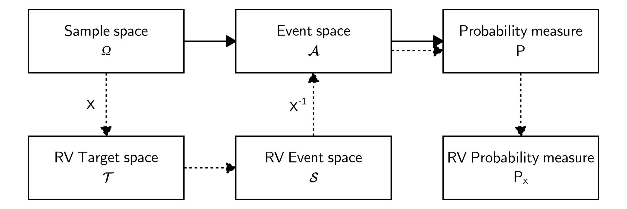
In machine learning, we often avoid explic- itly referring to the probability space, but instead refer to probabilities on quantities of interest, which we denote by \(\mathcal{T}\) . In this book, we refer to \(\mathcal{T}\) as the target space and refer to elements of \(\mathcal{T}\) as states. We introduce a function X : Ω → \(\mathcal{T}\) that takes an element of Ω (an event) and returns a particular quantity of interest x, a value in \(\mathcal{T}\) . This association/mapping from Ω to \(\mathcal{T}\) is called a random variable.
We need a mapping \(\mathcal{T}\): \[\Omega\stackrel{X}{\longrightarrow}\mathcal{T}\]
For any subset \(S \subseteq \mathcal{T}\) , we associate \(P_X(S) \in [0, 1]\) (the probability) to a particular event occurring corresponding to the random variable X.
7.2.1 Random variable: X
- quantity of interest: number of head
Python: Random variable and target space
X is \(X\); T_big is \(\mathcal{T}\)
7.2.2 Random variable event space: \(\mathcal{S}\)
For any subset \(S \subseteq \mathcal{T}\)
Python: rv event space \(\mathcal{S}\)
Let \(\mathcal{S}\) denote all possible subsets of \(\mathcal{T}\), named it S_big.
7.2.3 Random variable probability: \(P_X\)
From MML (6.8): For \(S \subseteq \mathcal{T}\), we have the notation \[P_X(S)=P(X \in S)=P(X^{−1}(S))=P({\omega \in \Omega: X(\omega)\in S}).\]
Given the probability space, we should be able to
back track the event that a rv event represents;
attach it with probability.
Python: inverse rv event space
X_pd=X.to_frame()
X_pd.reset_index(inplace=True)
X_pd.columns=['index','T']
X_inverse=X_pd.set_index('T')["index"]- Find \(X\_inv\_S\_0=X^{-1}(S\_0)\) if \(S\_0=\)
frozenset({1, 2})usingX_inverse. (make the result as a frozenset.)
- Find \(X^{-1}(S)\) for all \(S\in \mathcal{S}\).
7.3 Graphical relationship
| A_big | P |
|---|---|
| frozenset({(‘t’, ‘h’)}) | 0.25 |
| frozenset({(‘h’, ‘h’), (‘h’, ‘t’), (‘t’, ‘t’)}) | 0.75 |
| frozenset({(‘t’, ‘h’), (‘h’, ‘h’)}) | 0.50 |
| frozenset({(‘t’, ‘h’), (‘h’, ‘h’), (‘h’, ‘t’)}) | 0.75 |
| frozenset({(‘t’, ‘h’), (‘h’, ‘h’), (‘t’, ‘t’)}) | 0.75 |
| frozenset({(‘t’, ‘h’), (‘h’, ‘h’), (‘h’, ‘t’), (‘t’, ‘t’)}) | 1.00 |
| frozenset({(‘h’, ‘h’), (‘t’, ‘t’)}) | 0.50 |
| frozenset({(‘h’, ‘t’)}) | 0.25 |
| frozenset({(‘t’, ‘t’)}) | 0.25 |
| frozenset({(‘h’, ‘t’), (‘t’, ‘t’)}) | 0.50 |
| frozenset({(‘h’, ‘h’), (‘h’, ‘t’)}) | 0.50 |
| frozenset({(‘t’, ‘h’), (‘h’, ‘t’), (‘t’, ‘t’)}) | 0.75 |
| frozenset({(‘h’, ‘h’)}) | 0.25 |
| frozenset({(‘t’, ‘h’), (‘h’, ‘t’)}) | 0.50 |
| frozenset() | 0.00 |
| frozenset({(‘t’, ‘h’), (‘t’, ‘t’)}) | 0.50 |
| S_big | X_inv | Px |
|---|---|---|
| frozenset({2}) | frozenset({(‘h’, ‘h’)}) | 0.25 |
| frozenset({0, 1, 2}) | frozenset({(‘h’, ‘t’), (‘h’, ‘h’), (‘t’, ‘h’), (‘t’, ‘t’)}) | 1.00 |
| frozenset({1, 2}) | frozenset({(‘h’, ‘t’), (‘t’, ‘h’), (‘h’, ‘h’)}) | 0.75 |
| frozenset({0, 1}) | frozenset({(‘h’, ‘t’), (‘t’, ‘h’), (‘t’, ‘t’)}) | 0.75 |
| frozenset({0, 2}) | frozenset({(‘h’, ‘h’), (‘t’, ‘t’)}) | 0.50 |
| frozenset({1}) | frozenset({(‘h’, ‘t’), (‘t’, ‘h’)}) | 0.50 |
| frozenset() | frozenset() | 0.00 |
| frozenset({0}) | frozenset({(‘t’, ‘t’)}) | 0.25 |
找出A_big中不在X_inverse_S_big的集合collection.
7.4 Bayesian Theorem
\[ \Pr(\theta|\mbox{Sample})=\frac{\Pr(\mbox{Sample}|\theta)\Pr(\theta)}{\Pr(\mbox{Sample})} \]
Where:
Prior: \(\Pr(\theta)\)
Posterior: \(\Pr(\theta|\mbox{Sample})\)
Likelihood: \(\Pr(\mbox{Sample}|\theta)\), we normally write it as \(L(\theta|\mbox{Sample})\)
Note that \(\Pr(\mbox{Sample})\) is an unconditional probability of Sample, which is irrelevant to \(\theta\) values. Therefore, there is a proportional relationship between \(\Pr(\theta|\mbox{Sample})\) and \(L(\theta|\mbox{Sample})\Pr(\theta)\), commonly expressed as: \[ \Pr(\theta|\mbox{Sample})\propto L(\theta|\mbox{Sample})\Pr(\theta). \] \(\propto\) means proportional to.
7.4.1 Likelihood
\[\Pr(\mbox{Sample}|\theta)\] is determined by:
- how we think data are generated?
Tossing a coin 100 times.
Sample is the outcomes of 100 trials, say \(\{y_i\}_{i=1}^{100}\) and \(y_i=1\) if it is head.
Given \(Y_i\stackrel{iid}{\sim} Bernoulli(p)\),
what is \(\Pr(\mbox{Sample}|\theta)\)?
Write a function that can generate a sample of 100 trials:
def sample_bernoulli(p,size):
    """p: <class 'float'>
       size: <class 'int'>"""
    ....
    return <sample of class numpy.ndarray>
Write a likelihood function for Bernoulli sample:
def likelihood_bernoulli(Sample,p):
    """Sample: <class numpy.ndarray>
       p: <class 'float'>
    """

    ...
    return <likelihood value of class 'float'>
7.4.2 Posterior distribution
Suppose prior \(\Pr(p=0.1)=0.3,\ \Pr(p=0.3)=0.7\). What would be the posterior \(\Pr(p|\mbox{Sample})\)
善用unpacking訂義prior distribution
Write a function represent the scaled posterior
def posterior_scaled(Sample, prior):
  """Sample: <class 'numpy.ndarray'>
     prior: <class 'numpy.ndarray'>
     """
  ...
  return <posterior_scaled, class 'numpy.ndarray'>
7.4.3 MLE vs. Bayesian estimation
Max.Likelihood: To max \(L(\theta|\mbox{Sample})\)
Bayesian: To max \(\mathbf{E}(Loss(\hat{\theta},\theta)|Sample)\) with a posterioir probability of \(\Pr(\theta|\mbox{Sample})\).
令 \[Loss(\theta)=(\hat{\theta}-\theta)^2\] 求Bayesian estimate
7.4.4 Conjugacy
- MML 6.6
A prior is conjugate for the likelihood function if the posterior is of the same form/type as the prior.