Brief introduction to Statistic
Daxue Consulting
1 Methods for Describing a Set of Data
1.1 Numerical measure of Central Tendency
When we speak of a data set, we refer to either a sample or a population. If statistical inference is our goal, we’ll wish ultimately to use sample numerical descriptive measures to make inferences about the corresponding measures for the population.
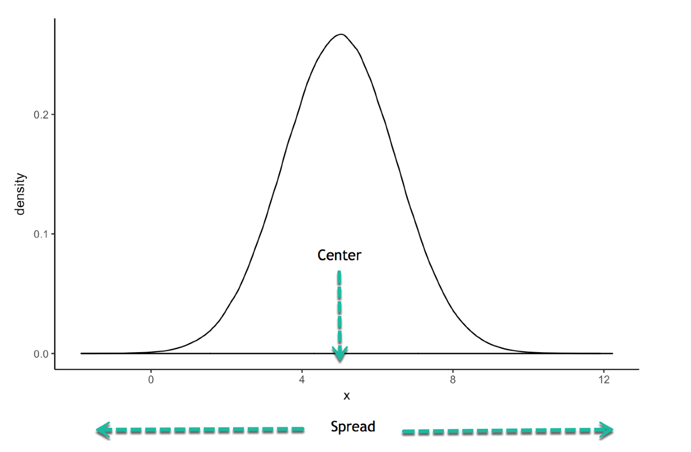
- The central tendency of the set of measurements: the tendency of the data to cluster, or center, about certain numerical values
- The variability of the set of measurements: the spread of the data
1.1.1 Measure of central tendency
- Mean
The **mean** of a set of quantitative data is the sum of the measurements divided by the number of measurements contained in the data set.The sample mean, \(\bar{x}\), will play an important role in accomplishing our objective of making inferences about populations based on sample information.
For this reason, we need to use a different symbol for the mean of a population.
- \(\bar{x}\): sample mean
- \(\mu\): Population mean
We’ll often use the sample mean \(\bar{x}\) to estimate (make an inference about) the population mean, \(\mu\).
Example
For example, the percentages of revenues spent on R&D by the population consisting of all U.S. companies has a mean equal to some value, \(\mu\).
Our sample of 50 companies yielded percentages with a mean of \(\bar{x}\) = 8.492. If, as is usually the case, we don’t have access to the measurements for the entire population, we could use \(\bar{x}\) as an estimator or approximator for \(\mu\).
Then we’d need to know something about the reliability of our inference-that is, we’d need to know how accurately we might expect \(\bar{x}\) to estimate \(\mu\)
In next tutorial, we’ll find that this accuracy depends on two factors:
- The size of the sample. The larger the sample, the more accurate the estimate will tend to be.
- The variability, or spread, of the data. All other factors remaining constant, the more variable the data, the less accurate the estimate.
Median
The median of a quantitative data set is the middle number when the measurements are arranged in ascending (or descending) order.In certain situations, the median may be a better measure of central tendency than the mean. In particular, the median is less sensitive than the mean to extremely large or small measurements.
A data set is said to be skewed if one tail of the distribution has more extreme observations than the other tail.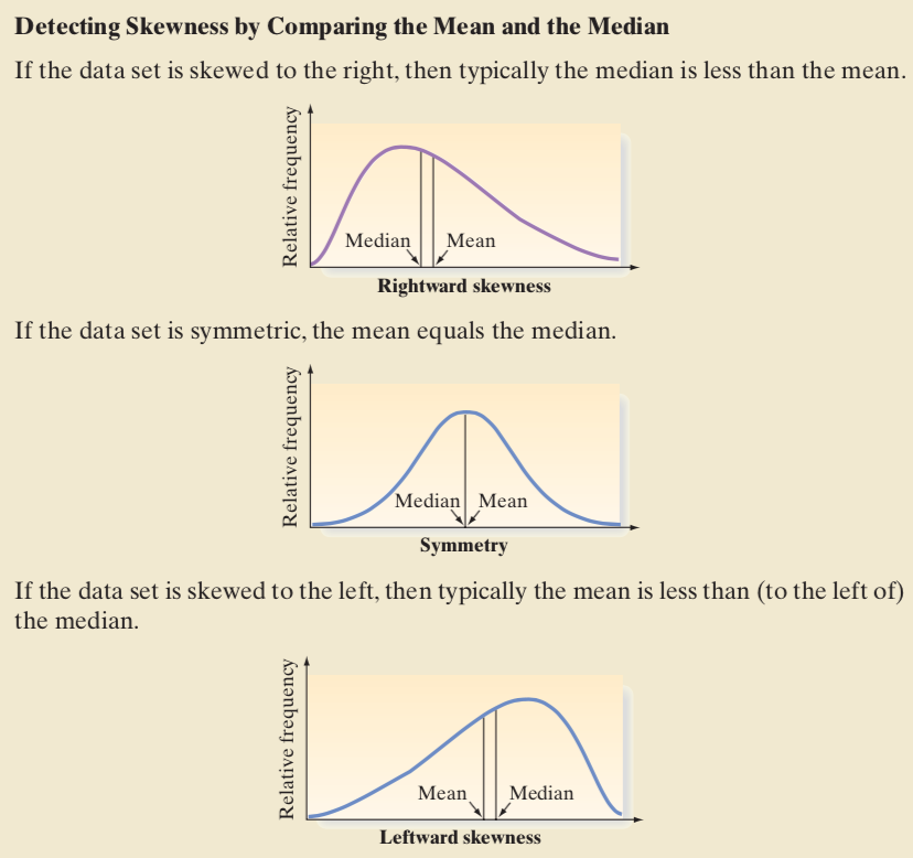
Mode
The mode is the measurement that occurs most frequently in the data set.1.1.2 Numerical Measures of Variability
Measures of central tendency provide only a partial description of a quantitative data set. The description is incomplete without a measure of the variability, or spread, of the data set.
Knowledge of the data’s variability along with its center can help us visualize the shape of a data set as well as its extreme values.
The sample variance for a sample of n measurements is equal to the sum of the squared deviations from the mean divided by (n - 1).Formula
\[ \sigma^2 = \frac{\sum(x_i- \bar{x})^2}{n-1} \] Note: that the population vairance is \[\sigma^2 = \frac{\sum(x_i- \mu)^2}{N}\]
The second step in finding a meaningful measure of data variability is to calculate the standard deviation of the data set.
The sample standard deviation is defined as the positive square root of the sample varianceNotice that, unlike the variance, the standard deviation is expressed in the original units of measurement. For example, if the original measurements are in dollars, the variance is expressed in the peculiar units “dollars squared”“, but the standard deviation is expressed in dollars.
You may wonder why we use the divisor \((n - 1)\) instead of \(n\) when calculating the sample variance. Wouldn’t using \(n\) be more logical so that the sample variance would be the average squared deviation from the mean?
The trouble is that using \(n\) tends to produce an underestimate of the population variance so we use \((n - 1)\) in the denominator to provide the appropriate correction for this tendency.
You now know that the standard deviation measures the variability of a set of data.
- The larger the standard deviation, the more variable the data.
- The smaller the standard deviation the less variable the data
1.1.3 Using the Mean and Standard Deviation to Describe Data
We’ve seen that if we are comparing the variability of two samples selected from a population, the sample with the larger standard deviation is the more variable of the two. Thus, we know how to interpret the standard deviation on a relative or comparative basis, but we haven’t explained how it provides a measure of variability for a single sample.
To understand how the standard deviation provides a measure of variability of a data set, consider a specific data set and answer the following questions:
- How many measurements are within 1 standard deviation of the mean?
- How many measurements are within 2 standard deviations?
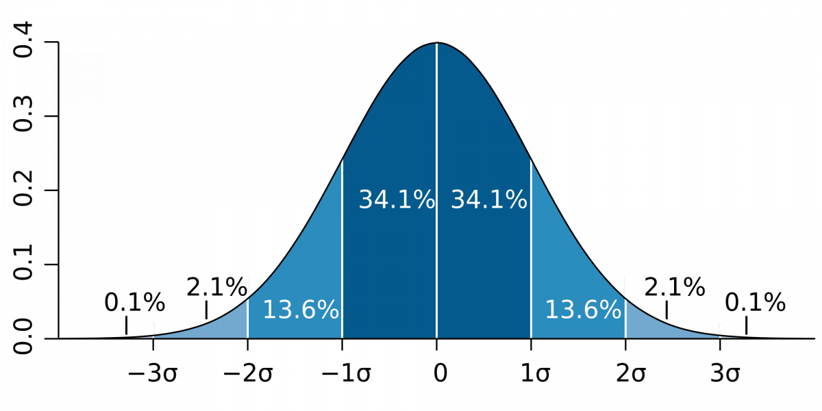
The Empirical Rule is a rule of thumb that applies to data sets with frequency distributions that are mound-shaped and symmetric, as shown below.
- Approximately 68% of the measurements willfall within 1 standard deviation of the mean
- Approximately 95% of the measurements will fall within 2 standard deviations of the mean
- Approximately 99.7% (essentially all) of the measurements will fall within 3 standard deviations of the mean
Example
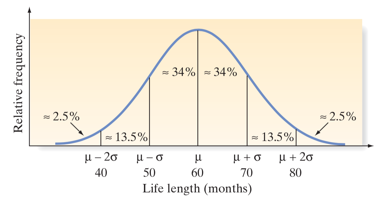
A manufacturer of automobile batteries claims that the average length of life for its grade A battery is 60 months. However, the guarantee on this brand is for just 36 months. Suppose the standard deviation of the life length is known to be 10 months, and the frequency distribution of the life-length data is known to be mound-shaped.
- Approximately what percentage of the manufacturer’s grade A batteries will last more than 50 months, assuming the manufacturer’s claim is true?
- Approximately what percentage of the manufacturer’s batteries will last less than 40 months, assuming the manufacturer’s claim is true?
- Suppose your battery lasts 37 months. What could you infer about the manufacturer’s claim?
Answer
- It is easy to see that the percentage of batteries lasting more than 50 months is approximately 34% (between 50 and 60 months) plus 50% (greater than 60 months). Thus, approximately 84% of the batteries should have life length exceeding 50 months.
- The percentage of batteries that last less than 40 months can also be easily determined. Approximately 2.5% of the batteries should fail prior to 40 months, assuming the manufacturer’s claim is true.
- If you are so unfortunate that your grade A battery fails at 37 months, you can make one of two inferences: either your battery was one of the approximately 2.5% that fail prior to 40 months, or something about the manufacturer’s claim is not true. Because the chances are so small that a battery fails before 40 months, you would have good reason to have serious doubts about the manufacturer’s claim. A mean smaller than 60 months and/or a standard deviation longer than 10 months would both increase the likelihood of failure prior to 40 months.
1.2 Numerical Measures of Relative Standing
Another measure of relative standing in popular use is the z-score. As you can see in the definition of z-score below, the z-score makes use of the mean and standard deviation of the data set in order to specify the relative location of a measurement. Note that the z-score is calculated by subtracting \(\bar{x}\) (or \(\mu\)) from the measurement \(x\) and then dividing the result by \(s\) (or \(\sigma\)). The final result, the z-score, represents the distance between a given measurement \(x\) and the mean, expressed in standard deviations.
\[ z = \frac{x-\bar{x}}{s} \]
with \(s\) is the sample sd
\[ z = \frac{x-\mu}{\sigma} \]
Example
A random sample of 2,000 students who sat for the Graduate Management Admission Test (GMAT) is selected.
For this sample, the mean GMAT score is \(x\) = 540 points and the standard deviation is \(s\) = 100 points.
One student from the sample, Kara Smith, had a GMAT score of \(x\) = 440 points. What is Kara’s sample z-score?
(440-540)/100## [1] -1This z-score implies that Kara Smith’s GMAT score is 1.0 standard deviations below the sample mean GMAT score, or, in short, her sample z-score is - 1.0.
Interpretation of z-Scores for Mound-Shaped Distributions of Data
- Approximately 68% of the measurements will have a z-score between -1 and 1.
- Approximately 95% of the measurements will have a z-score between - 2 and 2.
- Approximately 99.7% (almost all) of the measurements will have a z-score between -3 and 3.