3 Discrete Random Variables

3.1 Probability Distribution for Discrete Random Variables

A complete description of a discrete random variable requires that we specify the possible values the random variable can assume and the probability associated with each value.

The probability distribution of a discrete random variable is a graph, table, or formula that specifies the probability associated with each possible value the random variable can assume.

Imagine we toss two coins. The random variable \(x\) can assume values 0, 1, and 2. What is the probability of:

\[ P(x=0) = P(TT) \] \[ P(x=1) = P(TH) + P(HT) \] \[ P(x=2) = P(HH) \] \[ T= tail \] \[ H = Head \]

TT <- 1/4
TH <- 1/4 + 1/4
HH <- 1/4
print(paste("TT=", TT, ", TH=", TH, ", HH=", HH))

## [1] "TT= 0.25 , TH= 0.5 , HH= 0.25"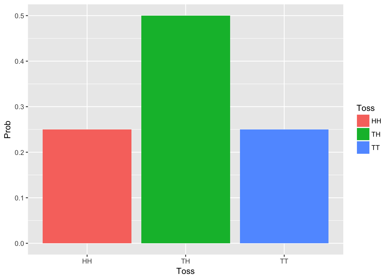

The probabilities as the heights of vertical lines over the corresponding values of \(x\).

Mean of a discrete random variable

To get the population mean of the random variable \(x\), we multiply each possible value of \(x\) by its probability \(p(x)\) and then sum this product over all possible values of x. The mean of x is also referred to as the expected value of x, denoted \(E(x)\).

\[ \mu = E(x) = \sum{xp(x)} \]

Example

Suppose you work for an insurance company, and you sell a 10,000 one- year term insurance policy at an annual premium of 290. Actuarial tables show that the probability of death during the next year for a person of your customer’s age, sex, health, etc., is .001.

What is the expected gain (amount of money made by the company) for a policy of this type?

290*.999 + (9710)*.001

## [1] 299.42

Variance of a discrete random variable

The population variance \(\sigma^2\) is defined as the average of the squared distance of \(x\) from the population mean \(\mu\). Because \(x\) is a random variable, the squared distance, \((x - \mu)^2\), is also a random variable.

\[ \sigma^2 = E[(x-\sigma)^2] = \sum(x-\mu)^2p(x) \] The standard deviation of x is defined as the square root of the variance \(\sigma^2\).

Example

Suppose you invest a fixed sum of money in each of five Internet business ventures.

Assume you know that 70% of such ventures are successful, the outcomes of the ventures are independent of one another, and the probability distribution for the number, \(x\), of successful ventures out of five is:

x	0	1	2	3	4	5
p(x)	0,002	0,029	0,132	0,309	0,36	0,168

Find \(\mu\)
Find \(\sigma\)

Answers

0*.002+1*.029+2*.132+3*.309+4*.360+5*.168

## [1] 3.5

On average, the number of successful ventures out of five will equal 3.5

(0-3.5)^2*.002 + (1-3.5)^2*.029+ (2-3.5)^2*.132+(3-3.5)^2*.309+(4-3.5)^2*.360+(5-3.5)^2*.168

## [1] 1.048

3.2 The Binomial Distribution

Many experiments result in dichotomous responses. It means responses for which there exist two possible alternatives, such as Yes-No, Pass-Fail, Defective-Nondefective, or Male-Female.

Formula

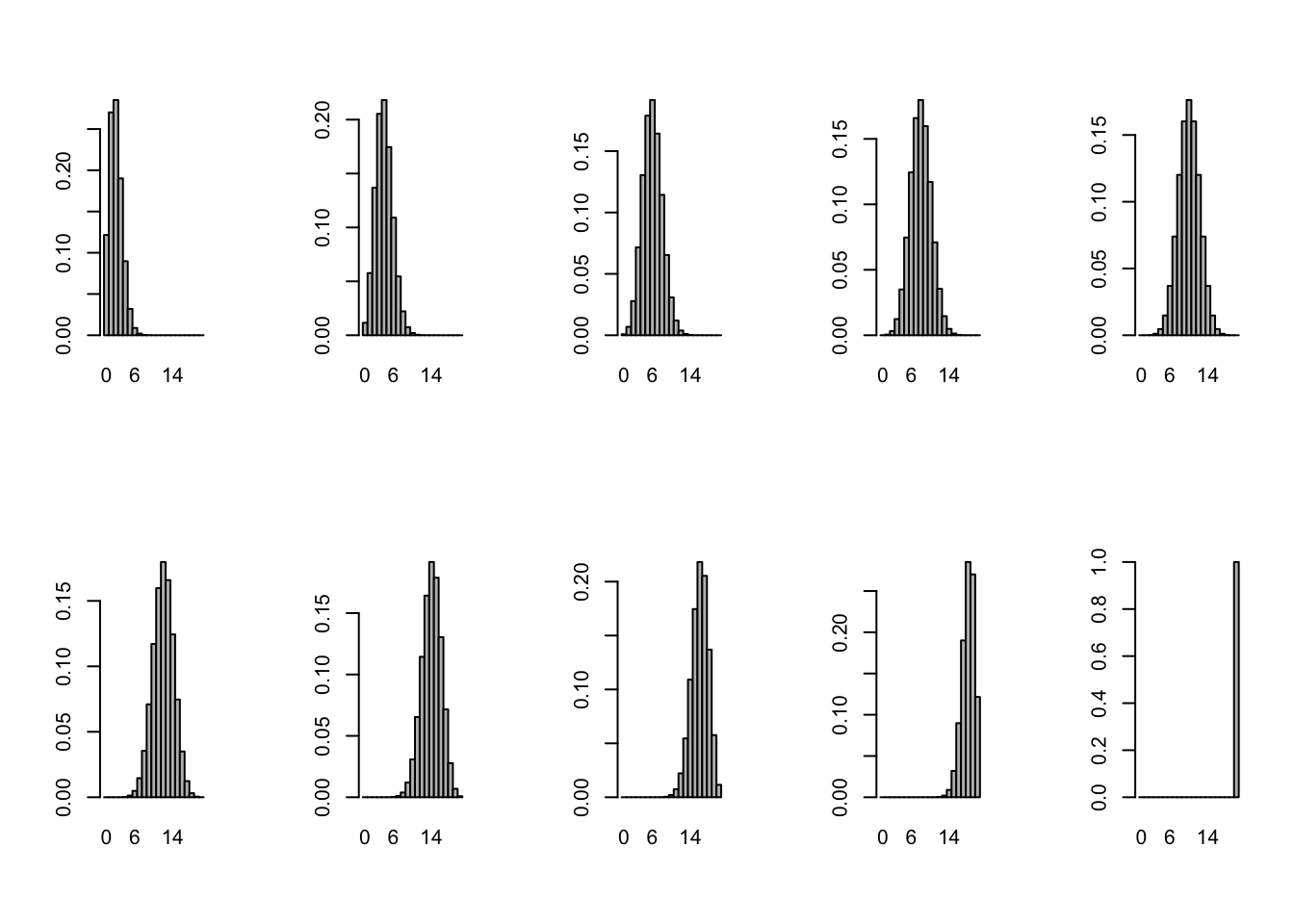
\[ p(x) = \binom{n}{x}p^xq^{n-x} \] with:

\(p\) = Probability of success on a single trial \(q\) = 1-\(p\) \(n\) = Number of trials \(x\) = Number of successess in \(n\) trials \(n-x\)= Number of failures in \(n\) trials \[\binom{n}{x} = \frac{n!}{x!(n-x)!}\]

par(mfrow=c(2, 5))
for(p in seq(0.1, 1, len=10))
{
    x <- dbinom(0:20, size=20, p=p)
    barplot(x, names.arg=0:20, space=0)
}

A simple example of such an experiment is the coin-toss experiment. A coin is tossed a number of times, say 10. Each toss results in one of two outcomes, Head or Tail. Ultimately, we are interested in the probability distribution of \(x\), the number of heads observed. Many other experiments are equivalent to tossing a coin (either balanced or unbalanced) a fixed number \(n\) of times and observing the number \(x\) of times that one of the two possible outcomes occurs.

Random variables that possess these characteristics are called binomial random variables.

Survey frequently yields observations on binomial random variables. For example, suppose a sample of 100 current customers is selected from a firm’s database and each person is asked whether he or she prefers the firm’s product (a Head) or prefers a competitor’s product (a Tail). Suppose we are interested in \(x\), the number of customers in the sample who prefer the firm’s product. Sampling 100 customers is analogous to tossing the coin 100 times.

Example

Suppose there are twelve multiple choice questions in an English class quiz. Each question has five possible answers, and only one of them is correct. Find the probability of having four or less correct answers if a student attempts to answer every question at random.

Since only one out of five possible answers is correct, the probability of answering a question correctly by random is 1/5=0.2. We can find the probability of having exactly 4 correct answers by random attempts as follows.

dbinom(4, size=12, prob=0.2)

## [1] 0.1328756

To find the probability of having four or less correct answers by random attempts, we apply the function dbinom with x = 0,…,4.

dbinom(0, size=12, prob=0.2) + 
dbinom(1, size=12, prob=0.2) + 
dbinom(2, size=12, prob=0.2) + 
dbinom(3, size=12, prob=0.2) + 
dbinom(4, size=12, prob=0.2)

## [1] 0.9274445

Alternatively, we can use the cumulative probability function for binomial distribution pbinom.

pbinom(4, size=12, prob=0.2)

## [1] 0.9274445

The probability of four or less questions answered correctly by random in a twelve question multiple choice quiz is 92.7%.

3.3 Other discrete Distribution

3.3.1 Poisson

A type of discrete probability distribution that is often useful in describing the number of rare events that will occur in a specific period of time or in a specific area or volume is the Poisson distribution

Formula

\[ p(x) = \frac{\lambda ^xe^{-\lambda}}{x!} \]

with \(\mu=\lambda\) = mean number of events during given unit of time, area

Example

The number of industrial accidents per month at a manufacturing plant
The number of noticeable surface defects (scratches, dents, etc.) found by quality inspectors on a new automobile
The parts per million of some toxin found in the water or air emission from a manufacturing plant
The number of customer arrivals per unit of time at a supermarket checkout counter

If there are twelve cars crossing a bridge per minute on average, find the probability of having seventeen or more cars crossing the bridge in a particular minute.

The probability of having sixteen or less cars crossing the bridge in a particular minute is given by the function ppois.

ppois(16, lambda=12)   # lower tail

## [1] 0.898709

Hence the probability of having seventeen or more cars crossing the bridge in a minute is in the upper tail of the probability density function.

ppois(16, lambda=12, lower=FALSE)   # upper tail

## [1] 0.101291

If there are twelve cars crossing a bridge per minute on average, the probability of having seventeen or more cars crossing the bridge in a particular minute is 10.1%.