5 Estimation with confidence intervals
In this tutorial, our goal is to estimate the value of an unknown population parameter, such as a population mean or a proportion from a binomial population. For example, we might want to know the mean gas mileage for a new car model, the average expected life of a flat-screen computer monitor, or the proportion of dot-com companies that fail within a year of start-up.
We want to use the sample information to estimate the population parameter of interest (called the target parameter) and assess the reliability of the estimate.
The unknown population parameter (e.g., mean or proportion) that we are interested in estimating is called the target parameter.For the examples given above, the words mean in mean gas mileage and average in average life expectancy imply that the target parameter is the population mean, \(\mu\). The word proportion in proportion of dot-com companies that fail within one year of start-up indicates that the target parameter is the binomial proportion, \(p\).
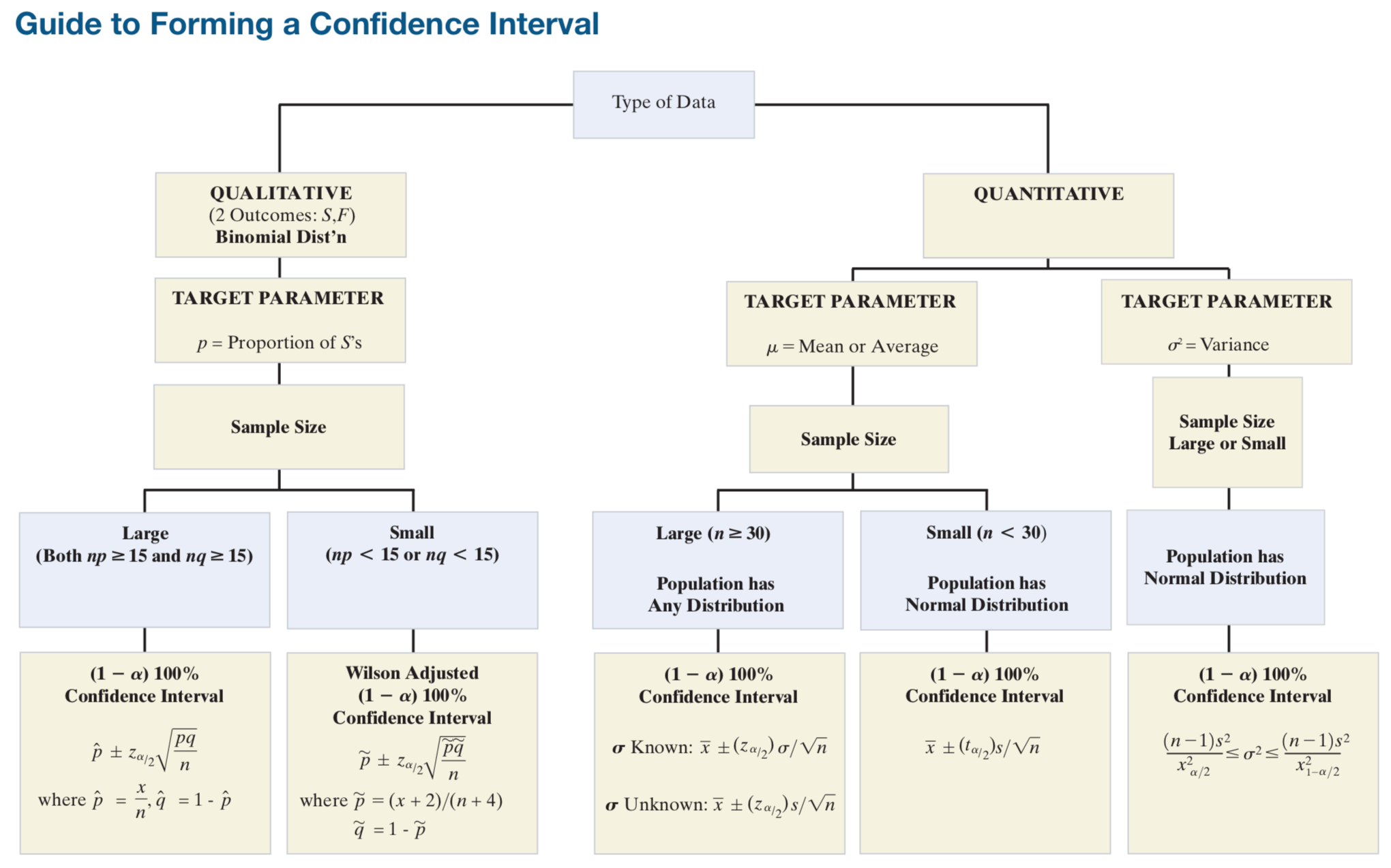
In addition to key words and phrases, the type of data (quantitative or qualitative) collected is indicative of the target parameter.
With quantitative data, you are likely to be estimating the mean or variance of the data.
With qualitative data with two outcomes (success or failure), the binomial proportion of successes is likely to be the parameter of interest.
A single number calculated from the sample that estimates a target population parameter is called a point estimator.
For example, we’ll use the sample mean, \(\bar{x}\), to estimate the population mean \(\mu\). Consequently, \(\bar{x}\) is a point estimator.
Similarly, we’ll learn that the sample proportion of successes, denoted \(\hat{p}\), is a point estimator for the binomial proportion \(p\) and that the sample variance \(s^2\) is a point estimator for the population variance \(\sigma\).
We will attach a measure of reliability to our estimate by obtaining an interval estimator-a range of numbers that contain the target parameter with a high degree of confidence.
For this reason the interval estimate is also called a confidence interval.
A point estimator of a population parameter is a rule or formula that tells us how to use the sample data to calculate a single number that can be used as an estimate of the target parameter.An interval estimator (or confidence interval) is a formula that tells us how to use the sample data to calculate an interval that estimates the target parameter.5.1 Confidence Interval for a Population Mean: Normal (z) Statistic (known Variance)
According to the Central Limit Theorem, the sampling distribution of the sample mean is approximately normal for large samples. The formula is
\[ \bar{x}+/-\frac{1.96*\sigma}{\sqrt{n}} \]
That is, we form an interval from 1.96 standard deviations below the sample mean to 1.96 standard deviations above the mean.
Example
Consider the large bank that wants to estimate the average amount of money owed by its delinquent debtors, \(m\). The bank randomly samples \(n = 100\) of its delinquent accounts and finds that the sample mean amount owed is \(\bar{x} = 230\). Also, suppose it is known that the standard deviation of the amount owed for all delinquent accounts is \(\sigma = +90\).
Calculate a confidence interval for the target parameter, \(m\).
230 + (1.96*90)/sqrt(100)## [1] 247.64230 - (1.96*90)/sqrt(100)## [1] 212.36The confidence coefficient is the probability that a randomly selected confidence interval encloses the population parameter’that is, the relative frequency with which similarly constructed intervals enclose the population parameter when the estimator is used repeatedly a very large number of times. The confidence level is the confidence coefficient expressed as a percentage.
Note: Empirical research suggests that a sample size n exceeding a value between 20 and 30 will usually yield a sam- pling distribution of x that is approximately normal. This result led many practitioners to adopt the rule of thumb that a sample size of n > 30 is required to use large-sample confidence interval procedures
Summary
Usual value of \(z\)
- \(z_{99}\)= 2.576
- \(z_{95}\)= 2.326
- \(z_{90}\)= 1.645
Large sample Confidence Interval for M, Based on a Normal (z) Statistic
When \(\sigma\) is known
\[ \bar{x}+/-z*\frac{\sigma}{\sqrt{n}} \]
When \(\sigma\) is unknown
\[ \bar{x}+/-z*\frac{s}{\sqrt{n}} \] The sample size \(n\) is large (i.e., n > 30). Due to the Central Limit Theorem, this condition guarantees that the sampling distribution of \(x\) is approximately normal. (Also, for large \(n\), \(s\) will be a good estimator of \(\sigma\).)
Alternative
We can use the z.test from the library TeachingDemos
set.seed(123)
x <- rnorm(500)
n <- 500
x_bar <- mean(x)
sd <- sd(x)
left <- sd/sqrt(n)
E <- qnorm(.975)*left
x_bar + E
## [1] 0.1198559x_bar - E## [1] -0.05067498library(TeachingDemos)
z.test(x, sd = sd(x))##
## One Sample z-test
##
## data: x
## z = 0.79512, n = 500.000000, Std. Dev. = 0.972770, Std. Dev. of
## the sample mean = 0.043504, p-value = 0.4265
## alternative hypothesis: true mean is not equal to 0
## 95 percent confidence interval:
## -0.05067498 0.11985588
## sample estimates:
## mean of x
## 0.034590455.2 Confidence Interval for a Population Mean: Student’s t-Statistic (Unknown Variance)
Suppose a pharmaceutical company must estimate the average increase in blood pressure of patients who take a certain new drug. Assume that only six patients (randomly selected from the population of all patients) can be used in the initial phase of human testing. The use of a small sample in making an inference about m presents two immediate problems when we attempt to use the standard normal \(z\) as a test statistic.
2 problems
- The shape of the sampling distribution of the sample mean \(\bar{x}\) (and the z-statistic) now depends on the shape of the population that is sampled. We can no longer assume that the sampling distribution of \(\bar{x}\) is approximately normal because the Central Limit Theorem ensures normality only for samples that are sufficiently large.
- The population standard deviation \(\sigma\) is almost always unknown.
Solution, we can use the \(t\) distribution
Formula
\[ t= \frac{\bar{x} - \mu}{s/\sqrt{n}} \]
in which the sample standard deviation, \(s\), replaces the population standard deviation, \(\sigma\).
If we are sampling from a normal distribution, the t-statistic has a sampling distribution very much like that of the z-statistic: mound-shaped, symmetric, with mean 0. The primary difference between the sampling distributions of \(t\) and \(z\) is that the t-statistic is more variable than the \(z\), which follows intuitively when you realize that \(t\) contains two random quantities (\(x\) and \(\sigma\)), whereas \(z\) contains only one (\(x\)).
The actual amount of variability in the sampling distribution of \(t\) depends on the sample size \(n\).
Example
Consider the pharmaceutical company that desires an estimate of the mean increase in blood pressure of patients who take a new drug.
The blood pressure increases for the \(n = 6\) patients in the human testing phase. Use this information to construct a 95% confidence interval for \(\mu\), the mean increase in blood pressure associated with the new drug for all patients in the population.
The average increases is 2.283 and the sd is .949
First, note that we are dealing with a sample too small to assume that the sample mean \(x\) is approximately normally distributed by the Central Limit Theorem
Second, the variance is unknown.
To compute the CI with Student’s t-Statistic, we can cumpute
\[ \bar{x}=+/-t_{\sigma/2}\frac{s}{\sqrt{n}} \]
The value of \(t_{\sigma/2}\) in the Student table is 2.571 with \(n-1\) degree of freedom (6-1)
2.283 + 2.571*(0.950/sqrt(6))## [1] 3.2801262.283 - 2.571*(0.950/sqrt(6))## [1] 1.285874Small-Sample Confidence Interval for M, Student’s t-statistic
\(\sigma\) is unknwon
\[ \bar{x}+/-t_{\sigma/2}\frac{s}{\sqrt{n}} \]
\(\sigma\) is known
\[ \bar{x}+/-t_{\sigma/2}\frac{\sigma}{\sqrt{n}} \]
Alternative
We can use the t.test in the built-in stat package
set.seed(1234)
x <- rnorm(100)
t.test(x)
##
## One Sample t-test
##
## data: x
## t = -1.5607, df = 99, p-value = 0.1218
## alternative hypothesis: true mean is not equal to 0
## 95 percent confidence interval:
## -0.35605755 0.04253406
## sample estimates:
## mean of x
## -0.15676175.3 Sampling size of Population Mean
The quality of a sample survey can be improved by increasing the sample size. The formula below provide the sample size needed under the requirement of population mean interval estimate at \((1 - \alpha)\) confidence level, margin of error \(E\), and population variance \(z_{\alpha/2}\). Here, \(\sigma^2\) is the \(100(1- \alpha/2)\) percentile of the standard normal distribution.
\[ n = \frac{(z_{(\alpha/2)^2\sigma^2})}{E^2} \] example
Assume the population standard deviation \(\sigma\) of the student height in survey is 9.48. Find the sample size needed to achieve a 1.2 centimeters margin of error at 95% confidence level.
Since there are two tails of the normal distribution, the 95% confidence level would imply the 97.5th percentile of the normal distribution at the upper tail. Therefore, \(z_{\alpha/2}\) is given by qnorm(.975).
zstar = qnorm(.975)
sigma = 9.48
E = 1.2
zstar^2*sigma^2/E^2
## [1] 239.7454Based on the assumption of population standard deviation being 9.48, it needs a sample size of 240 to achieve a 1.2 centimeters margin of error at 95% confidence level.
5.4 Large-Sample Confidence Interval for a Population Proportion
In this part, we are interested in estimating the percentage (or proportion) of some group with a certain characteristic. In this section, we consider methods for mak- ing inferences about population proportions when the sample is large.
The formula to compute a large sample CI
\[ \hat{p}+/-z\sqrt{\frac{\hat{p}(1-\hat{p})}{n}} \]
with \(\hat{p} = x/n\)
Example
Many public polling agencies conduct surveys to determine the current consumer sentiment concerning the state of the economy. For example, the Bureau of Economic and Business Research (BEBR) at the University of Florida conducts quarterly surveys to gauge consumer sentiment in the Sunshine State.
Suppose that the BEBR randomly samples 484 consumers and finds that 157 are optimistic about the state of the economy. Use a 90% confidence interval to estimate the proportion of all consumers in Florida who are optimistic about the state of the economy.
We know \(x=484\) is the total consumers. \(z\) statistic at 90% is 1.645
p_hat <- 157/484
p_hat + 1.645*sqrt((.324*.676)/484)
## [1] 0.3593738p_hat - 1.645*sqrt((.324*.676)/484)## [1] 0.2893865Alternative
Compute the margin of error and estimate interval for the female students proportion in survey dataset at 95% confidence level.
library(MASS)
gender.response = na.omit(survey$Sex)
n = length(gender.response)    # valid responses count
k = sum(gender.response == "Female")
pbar = k/n
SE = sqrt(pbar*(1-pbar)/n)
E = qnorm(.975)*SE
pbar + c(-E, E)
## [1] 0.4362086 0.5637914prop.test(k, n) ##
## 1-sample proportions test without continuity correction
##
## data: k out of n, null probability 0.5
## X-squared = 0, df = 1, p-value = 1
## alternative hypothesis: true p is not equal to 0.5
## 95 percent confidence interval:
## 0.4367215 0.5632785
## sample estimates:
## p
## 0.5At 95% confidence level, between 43.6% and 56.3% of the university students are female, and the margin of error is 6.4%.
5.5 Sampling Size of Population Proportion
The quality of a sample survey can be improved by increasing the sample size. The formula below provide the sample size needed under the requirement of population proportion interval estimate at \((1- \sigma)\) confidence level, margin of error \(E\), and planned proportion estimate \(p\). Here, \(z_{\sigma/2}\) is the \(100(1 - \alpha/2)\) percentile of the standard normal distribution.
\[ n = \frac{(z_{\alpha/2)^2p(1-p)}}{E^2}) \] Example
Using a 50% planned proportion estimate, find the sample size needed to achieve 5% margin of error for the female student survey at 95% confidence level.
Since there are two tails of the normal distribution, the 95% confidence level would imply the 97.5th percentile of the normal distribution at the upper tail. Therefore, \(z\) is given by qnorm(.975).
zstar = qnorm(.975)
p = 0.5
E = 0.05
zstar^2 * p * (1-p) / E^2
## [1] 384.1459With a planned proportion estimate of 50% at 95% confidence level, it needs a sample size of 385 to achieve a 5% margin of error for the survey of female student proportion.