4 Continuous Random Variables
4.1 Probability Distributions for Continuous Random Variables
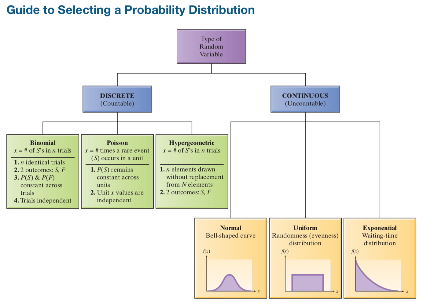
The graphical form of the probability distribution for a continuous random variable \(x\) is a smooth curve. This curve, a function of \(x\), is denoted by the symbol \(f(x)\) and is variously called a probability density function (pdf), a frequency function, or a probability distribution.
The probability distribution for a continuous random variable, x, can be represented by a smooth curve-a function of x, denoted f(x). The curve is called a density func- tion or frequency function. The probability that x falls between two values, a and b, i.e., P(a< x < b), is the area under the curve between a and b.4.2 The Normal Distribution
One of the most commonly observed continuous random variables has a bell-shaped probability distribution (or bell curve).
Formula
\[ f(x)= \frac{1}{\sigma \sqrt{2\pi }}e^{-1/2}[(x-\mu)/\sigma]^2 \]
We can transform the normal distribution in standard normal distribution with mean \(\mu = 0\) and sd \(\sigma =1\)
\[ f(x)= \frac{1}{\sigma \sqrt{2\pi }}e^{-1/2}z^2 \]
The normal distribution plays a very important role in the science of statistical inference. Moreover, many business phenomena generate random variables with probability distributions that are very well approximated by a normal distribution. For example, the monthly rate of return for a particular stock is approximately a normal random variable, and the probability distribution for the weekly sales of a corporation might be approximated by a normal probability distribution. The normal distribution might also provide an accurate model for the distribution of scores on an employment aptitude test.
Example
Assume that the test scores of a college entrance exam fits a normal distribution. Furthermore, the mean test score is 72, and the standard deviation is 15.2.
- What is the percentage of students scoring 84 or more in the exam?
We apply the function `pnorm of the normal distribution with mean 72 and standard deviation 15.2. Since we are looking for the percentage of students scoring higher than 84, we are interested in the upper tail of the normal distribution.
pnorm(84, mean=72, sd=15.2, lower.tail=FALSE) ## [1] 0.2149176The percentage of students scoring 84 or more in the college entrance exam is 21.5%.
Converting a Normal Distribution to a Standard Normal Distribution
If \(x\) is a normal random variable with mean m and standard deviation \(\sigma\), then the random variable \(z\), defined by the formula
\[ z = \frac{x-\mu}{\sigma} \]
Example
Suppose an automobile manufacturer introduces a new model that has an advertised mean in-city mileage of 27 miles per gallon. Although such advertisements seldom report any measure of variability, suppose you write the manufacturer for the details of the tests, and you find that the standard deviation is 3 miles per gallon.
This information leads you to formulate a probability model for the random variable \(x\), the in-city mileage for this car model. You believe that the probability distribution of x can be approximated by a normal distribution with a mean of 27 and a standard deviation of 3.
(20-27)/3## [1] -2.333333pnorm(-2.333) ## [1] 0.009824073According to this probability model, you should have only about a 1% chance of purchasing a car of this make with an in-city mileage under 20 miles per gallon.