8 Chi-squared Test of Independence
Many statistical quantities derived from data samples are found to follow the Chi-squared distribution. Hence we can use it to test whether a population fits a particular theoretical probability distribution.
8.1 Testing Category Probabilities: One-Way Table
In this section, we consider a multinomial experiment with k outcomes that correspond to categories of a single qualitative variable. The results of such an experiment are summarized in a one-way table. The term one-way is used because only one variable is classified. Typically, we want to make inferences about the true proportions that occur in the \(k\) categories based on the sample information in the one-way table.
A population is called multinomial if its data is categorical and belongs to a collection of discrete non-overlapping classes. Qualitative data that fall in more than two categories often result from a multinomial experiment. The characteristics for a multinomial experiment with \(k\) outcomes are described in the box.
Properties of the Multinomial Experiment

1. The experiment consists of n identical trials.
2. There are k possible outcomes to each trial. These outcomes are called classes, categories, or cells.
3. The probabilities of the k outcomes, denoted by p1, p2, c, pk, remain the same from trial to trial, where p1 + p2 + ... + pk = 1.
4. The trials are independent.
5. The random variables of interest are the cell counts, n1, n2, ..., nk, of the number of observations that fall in each of the k classes.
The chi-square goodness of fit test is used to compare the observed distribution to an expected distribution, in a situation where we have two or more categories in a discrete data. In other words, it compares multiple observed proportions to expected probabilities.
The null hypothesis for goodness of fit test for multinomial distribution is that the observed frequency fi is equal to an expected count \(e_i\) in each category. It is to be rejected if the p-value of the following Chi-squared test statistics is less than a given significance level \(\alpha\).
Formula
\[ \chi ^2=\sum \frac{(f_i-e_i)^2}{e_i} \]
Example
To illustrate, suppose a large supermarket chain conducts a consumer-preference survey by recording the brand of bread purchased by customers in its stores. Assume the chain carries three brands of bread: two major brands (A and B) and its own store brand. The brand preferences of a random sample of 150 consumers are observed, and the number preferring each brand is tabulated
| Brand | n |
|---|---|
| A | 61 |
| B | 53 |
| Store brand | 36 |
ncount <- c(61, 53, 36)
sum(ncount)
## [1] 150Note that our consumer-preference survey satisfies the properties of a multino- mial experiment for the qualitative variable brand of bread.
The experiment consists of randomly sampling \(n = 150\) buyers from a large population of consumers containing an unknown proportion \(p1\) who prefer brand A, a proportion \(p2\) who prefer brand B, and a proportion \(p3\) who prefer the store brand.
- H0: the brands of bread are equally preferred
- H1: At least one brand is preferred
res <- chisq.test(ncount)
res
##
## Chi-squared test for given probabilities
##
## data: ncount
## X-squared = 6.52, df = 2, p-value = 0.03839Since the computed \(\chi^2 = 6.52\) exceeds the critical value of 5.99147, we conclude at the \(\alpha = .05\) level of significance that a consumer preference exists for one or more of the brands of bread.
Example
For example, we collected wild tulips and found that 81 were red, 50 were yellow and 27 were white.
- Are these colors equally common?
If these colors were equally distributed, the expected proportion would be 1/3 for each of the color.
- Suppose that, in the region where you collected the data, the ratio of red, yellow and white tulip is 3:2:1 (3+2+1 = 6). This means that the expected proportion is:
- 3/6 (= 1/2) for red
- 2/6 ( = 1/3) for yellow
- 1/6 for white
We want to know, if there is any significant difference between the observed proportions and the expected proportions.
Statistical hypothesis
- Null hypothesis (H0): There is no significant difference between the observed and the expected value.
- Alternative hypothesis (H1): There is a significant difference between the observed and the expected value.
Answer
tulip <- c(81, 50, 27)
sum(tulip)
## [1] 158res <- chisq.test(tulip, p = c(1/3, 1/3, 1/3))
res##
## Chi-squared test for given probabilities
##
## data: tulip
## X-squared = 27.886, df = 2, p-value = 8.803e-07The p-value of the test is 8.80310^{-7}, which is less than the significance level alpha = 0.05. We can conclude that the colors are significantly not commonly distributed with a p-value = 8.80310^{-7}.
# Access to the expected values
res$expected
## [1] 52.66667 52.66667 52.66667tulip <- c(81, 50, 27)
res <- chisq.test(tulip, p = c(1/2, 1/3, 1/6))
res##
## Chi-squared test for given probabilities
##
## data: tulip
## X-squared = 0.20253, df = 2, p-value = 0.9037The p-value of the test is 0.9037, which is greater than the significance level alpha = 0.05. We can conclude that the observed proportions are not significantly different from the expected proportions.
8.2 Testing Category Probabilities: Two-Way (Contingency) Table
In previous section, we introduced the multinomial probability distribution and considered data classified according to a single qualitative criterion. We now consider multinomial experiments in which the data are classified according to two criteria. It means, classification with respect to two qualitative factors.
For example, consider a study published in the Journal of Marketing on the impact of using celebrities in television advertisements. The researchers investigated the rela- tionship between gender of a viewer and the viewer’s brand awareness. Three hundred TV viewers were asked to identify products advertised by male celebrity spokespersons.
| Awareness | Male | Female | total |
|---|---|---|---|
| identidy | 95 | 41 | 136 |
| no_identify | 50 | 114 | 164 |
| total | 145 | 155 | 300 |
df <- tribble(
  ~awareness, ~gender,~count,
  "identidy", "M", 95,
  "no_identify", "M",50,
  "identidy","F",41,
  "no_identify","F",114
)
df <- df %>% spread(gender, count)
df
## # A tibble: 2 x 3
## awareness F M
## * <chr> <dbl> <dbl>
## 1 identidy 41.0 95.0
## 2 no_identify 114 50.0Suppose we want to know whether the two classifications, gender and brand awareness, are dependent. If we know the gender of the TV viewer, does that information give us a clue about the viewer’s brand awareness?
chisq <- chisq.test(as.matrix(df[,2:3]))
chisq
##
## Pearson's Chi-squared test with Yates' continuity correction
##
## data: as.matrix(df[, 2:3])
## X-squared = 44.572, df = 1, p-value = 2.452e-11Large values of \(\chi\) imply that the observed counts do not closely agree, and hence, the hypothesis of independence is false.
Example 2
A large brokerage firm wants to determine whether the service it provides to affluent clients differs from the service it provides to lower-income clients. A sample of 500 clients is selected, and each client is asked to rate his or her broker.
| Broker rating | <30.000 | 30.000-60.000 | >60.000 | total |
|---|---|---|---|---|
| Outstanding | 48 | 64 | 41 | 153 |
| Average | 98 | 120 | 50 | 268 |
| Poor | 30 | 33 | 16 | 79 |
| total | 176 | 217 | 107 | 500 |
df <- tribble(
  ~Broker, ~income,~count,
  "Oustanding", "<30",48,
  "Avegare", "<30",98,
  "Poor","<30",30,
  "Oustanding", "30-60",64,
  "Avegare", "30-60",120,
  "Poor","30-60",33,
  "Oustanding", ">60",41,
  "Avegare", ">60",50,
  "Poor",">60",16
)

df <- df %>% spread(income, count)
df
## # A tibble: 3 x 4
## Broker `30-60` `<30` `>60`
## * <chr> <dbl> <dbl> <dbl>
## 1 Avegare 120 98.0 50.0
## 2 Oustanding 64.0 48.0 41.0
## 3 Poor 33.0 30.0 16.0chisq <- chisq.test(as.matrix(df[,2:4]))
chisq##
## Pearson's Chi-squared test
##
## data: as.matrix(df[, 2:4])
## X-squared = 4.2777, df = 4, p-value = 0.3697- Determine whether there is evidence that broker rating and customer income are dependent.
The null and alternative hypotheses we want to test are
- H0: The rating a client gives his or her broker is independent of client,s income.
- H1: Broker rating and client income are dependent.
This survey does not support the firm’s alternative hypothesis that affluent clients receive different broker service than lower-income clients.
8.3 Chi-squared Test of Independence
The chi-square test of independence is used to analyze the frequency table (i.e. contengency table) formed by two categorical variables. The chi-square test evaluates whether there is a significant association between the categories of the two variables.
file_path <- "http://www.sthda.com/sthda/RDoc/data/housetasks.txt"
housetasks <- read.delim(file_path, row.names = 1)
head(housetasks)
## Wife Alternating Husband Jointly
## Laundry 156 14 2 4
## Main_meal 124 20 5 4
## Dinner 77 11 7 13
## Breakfeast 82 36 15 7
## Tidying 53 11 1 57
## Dishes 32 24 4 53library("gplots")##
## Attaching package: 'gplots'## The following object is masked from 'package:stats':
##
## lowess# 1. convert the data as a table
dt <- as.table(as.matrix(housetasks))
# 2. Graph
balloonplot(t(dt), main ="housetasks", xlab ="", ylab="",
label = FALSE, show.margins = FALSE)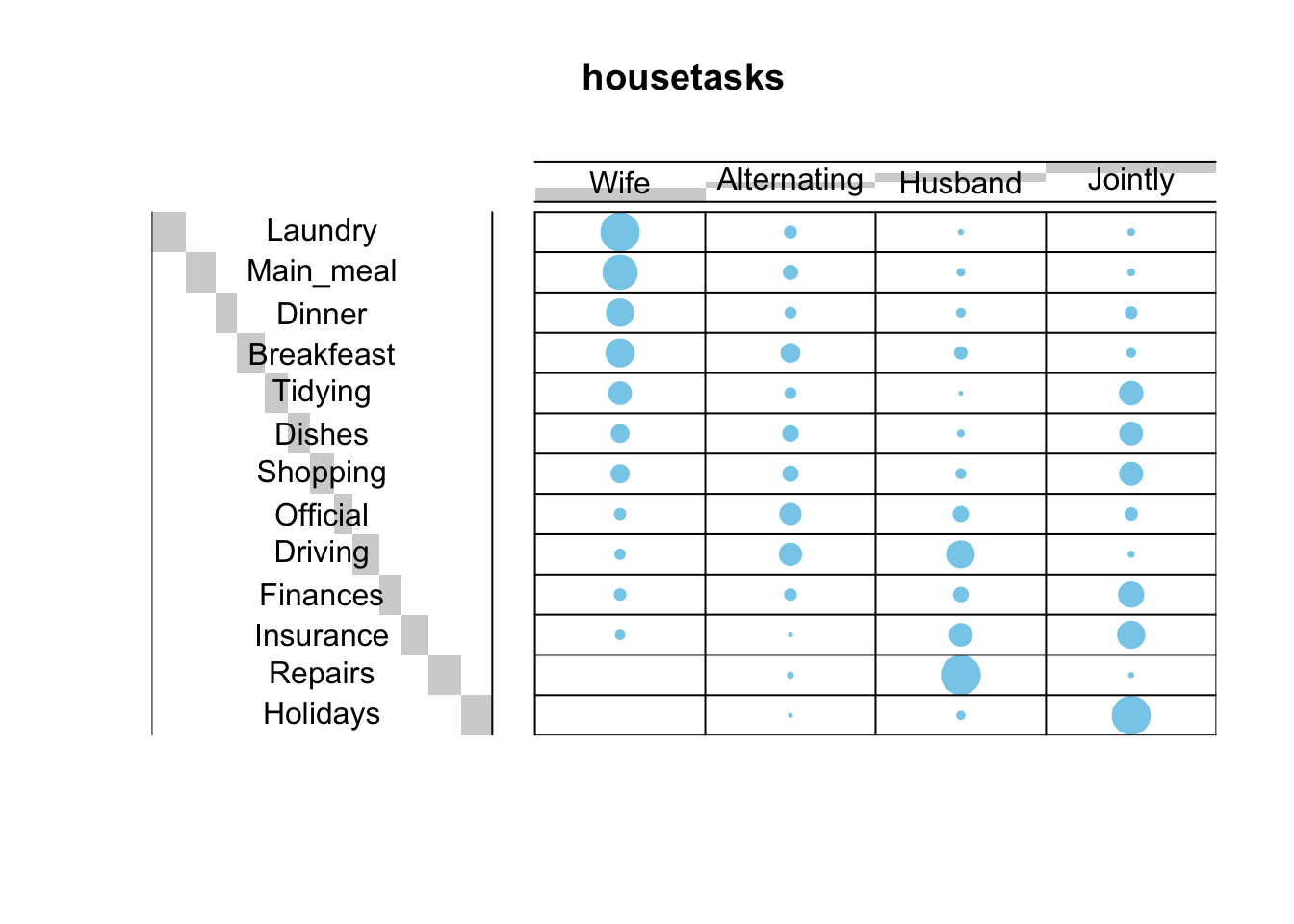
Chi-square test examines whether rows and columns of a contingency table are statistically significantly associated.
- Null hypothesis (H0): the row and the column variables of the contingency table are independent.
- Alternative hypothesis (H1): row and column variables are dependent
chisq <- chisq.test(housetasks)
chisq
##
## Pearson's Chi-squared test
##
## data: housetasks
## X-squared = 1944.5, df = 36, p-value < 2.2e-16In our example, the row and the column variables are statistically significantly associated (p-value = 0).
8.3.1 Nature of the dependence between the row and the column variables
If you want to know the most contributing cells to the total Chi-square score, you just have to calculate the Chi-square statistic for each cell: Pearson residuals (\(r\)) for each cell
library(corrplot)## corrplot 0.84 loaded# Contibution in percentage (%)
contrib <- 100*chisq$residuals^2/chisq$statistic
round(contrib, 3)## Wife Alternating Husband Jointly
## Laundry 7.738 0.272 1.777 2.246
## Main_meal 4.976 0.012 1.243 1.903
## Dinner 2.197 0.073 0.600 0.560
## Breakfeast 1.222 0.615 0.408 1.443
## Tidying 0.149 0.133 1.270 0.661
## Dishes 0.063 0.178 0.891 0.625
## Shopping 0.085 0.090 0.581 0.586
## Official 0.688 3.771 0.010 0.311
## Driving 1.538 2.403 3.374 1.789
## Finances 0.886 0.037 0.028 1.700
## Insurance 1.705 0.941 0.868 1.683
## Repairs 2.919 0.947 21.921 2.275
## Holidays 2.831 1.098 1.233 12.445corrplot(contrib, is.cor = FALSE)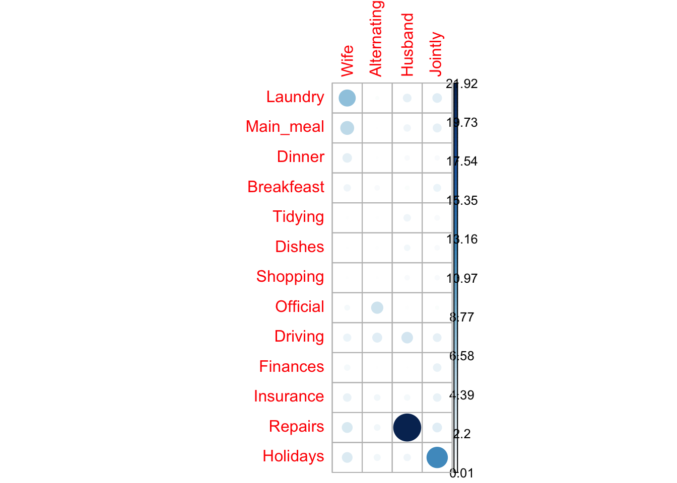
- In the image above, it’s evident that there are an association between the column Wife and the rows Laundry, Main_meal.
- There is a strong positive association between the column Husband and the row Repair