9 📝 Numerical Methods

9.1 Introduction to simulation

How can we determine the probability of winning a match in a card game?

The first method that comes to our mind consists in assuming that the \(52!\) permutations of the cards are equally likely, or use combinatorics.

Then, we “count” the number of favorable draws and divide by the \(52!\) = 8.0658175^{67} permutations.

• Unfortunately, the implementation of this criterion seems quite demanding: \(52!\) is a huge number.

• The computation of the required probability is hardly tractable from a strict mathematical standpoint…

However, we can decide to “drop” the rigorous mathematical treatment and invoke an approach which is pretty standard in the applied science:

we can simulate a game, that is we simulate an experiment.

For instance, in the case of card game, the experiment consists in playing a (very) large number of games and count the numbers of favorable events (cases where we draw the winning cards).

So, after the execution of \(n\) (say) games we will be able to set: \[X_i = \left\{\begin{array}{ll} 1& \mbox{ if the $i$-th game is a victory}\\ 0 & \mbox{ else} \end{array}\right.\] where the variables \(X_i\), for \(i=1,...n\) are random variables, each having a Bernoulli distribution such that \[E(X_i) = P(\text{win the card game}) = p.\]

Now, invoking the WLLN, we have that the proportion of won games converges, in probability to the probability of winning \(p\)

\[\bar{X}_n = \frac{\sum_{i=1}^n X_i}{n} = \frac{\text{# of favorable games}}{\text{# of total games played}} \overset{P}{\underset{n \to \infty}{\longrightarrow}} p\]

In words, we can claim that **after a large number of games the proportion of games that we win can be reasonably applied to get an estimate of \(p\).

Definition 1.1 The method which determines/estimates the probability (\(p\)) using experimentation (e.g., performing a long experiment in a computer, as in our example) is called simulation.

9.2 Simulation procedure

The remaining issue is that we have typically no time to play such a big number of games, so we let a computer play.

With this aim:

• We generate values from a random variable with a Uniform Distribution \(\mathcal{U}(0,1)\): these values are called random numbers.
• Starting from a \(U \sim \mathcal{U}(0,1)\) distribution, we can in principle simulate any random variable having a CDF, by means of the \(F^{-1}\) transformation.

\[F_U(u) = P(U \leq u) = \]

Remark. In fact, the computer makes use of the so called generator of pseudo random numbers: an algorithm produces a sequence of numbers which are (only) pseudo-random.

Namely, the generator yields a sequence of numbers that, practically, is very similar to a sample drawn form \(U(0,1)\). The way in which this algorithm works is behind the scope of this course: let’s simply say that you can use the statistical software to achieve the task.

9.3 Simulation in R

For instance, a well-know (freely available software) is R:

and 1 realization of a r.v \(\mathcal{B}(10, 0.5)\) can be obtained as:

rbinom(1, 10, 0.5)

## [1] 4

rbinom(1, 10, 0.5)

## [1] 6

rbinom(1, 10, 0.5)

## [1] 5

and 5 realization of a r.v.’s \(\mathcal{B}(10, 0.5)\) can be obtained as:

rbinom(5, 10, 0.5)

## [1] 3 7 7 3 7

rbinom(5, 10, 0.5)

## [1] 5 5 5 4 6

and 1 realization of a r.v.’s \(U(0, 1)\) can be obtained as:

runif(1, 0, 1)

## [1] 0.1808201

and 5 realization of a r.v.’s \(U(0, 1)\) can be obtained as:

runif(5, 0, 1)

## [1] 0.4052822 0.8535485 0.9763985 0.2258255 0.4448092

9.4 Coin tossing

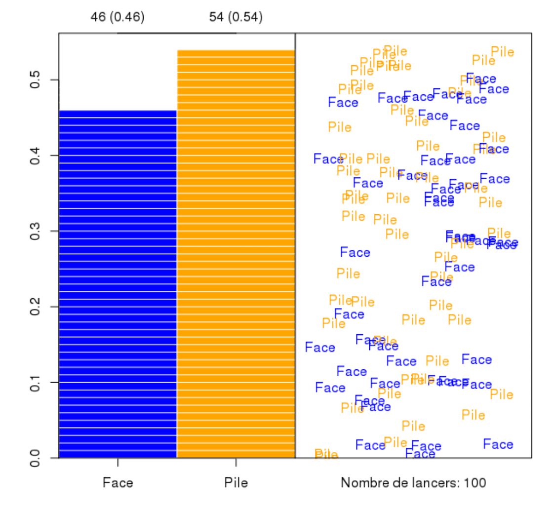
A computer cannot toss a coin, but it can generate Bernoulli random numbers so that we can simulate the outcomes of fair coin \(P(H)=P(T)=0.5\)

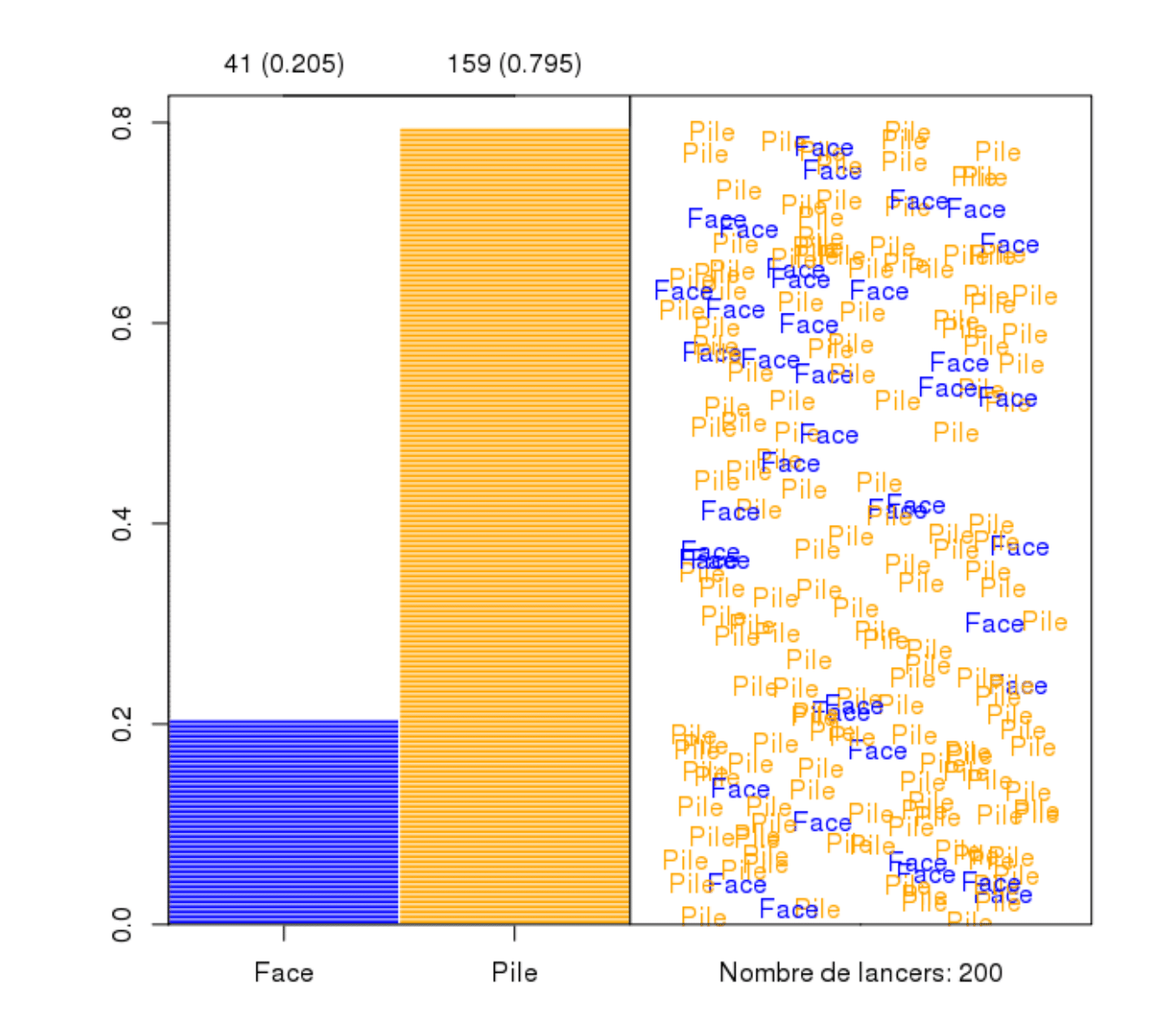
…or (exotic case) we can simulate the outcomes of unbalanced coin \(P(T)=0.8\)

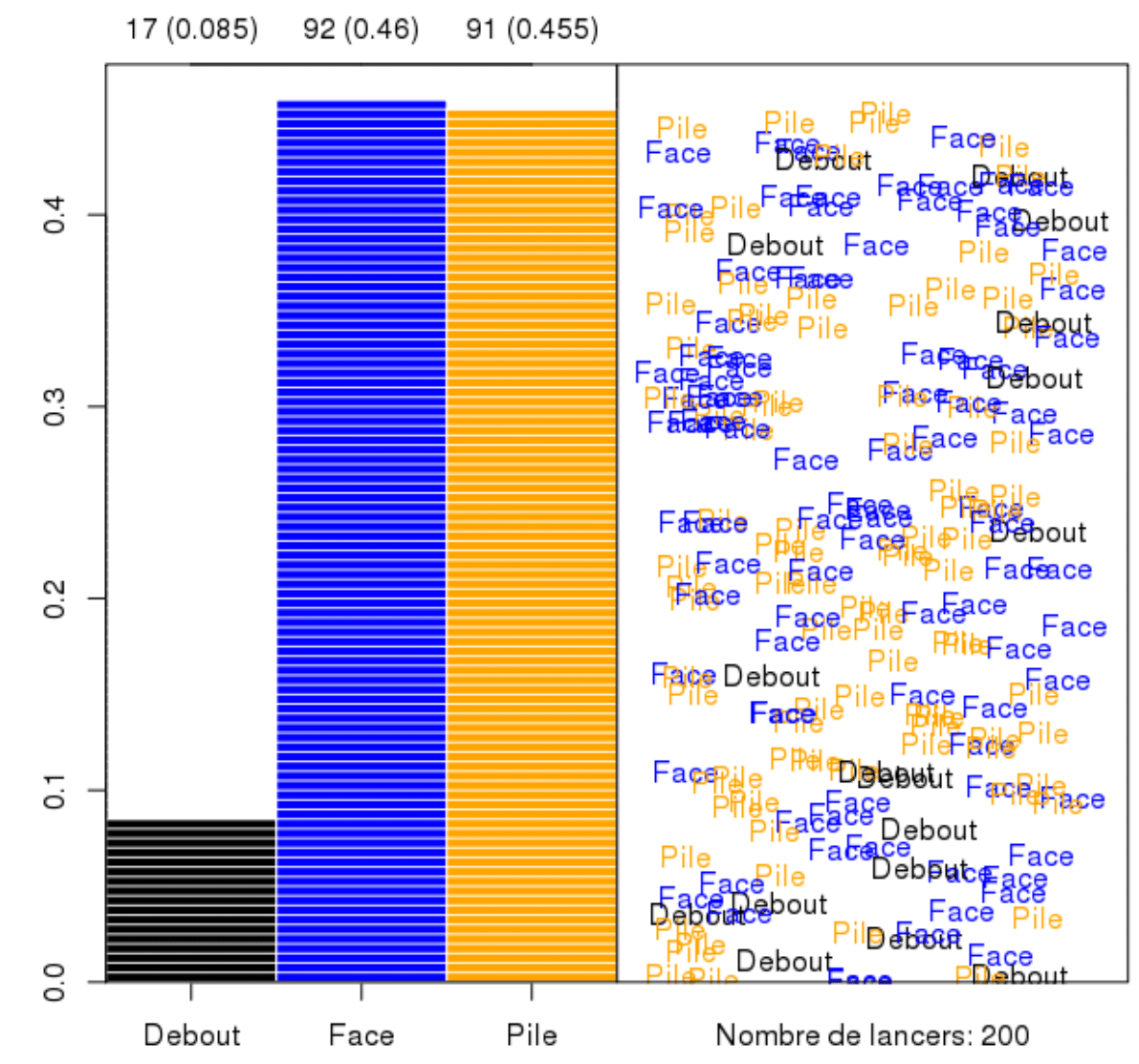
…or (even more exotic) we can simulate the outcomes of unbalanced coin \(P(H)=P(T)=0.45\) and probability of remaining on its edge \(0.1\)

9.5 Summarising

Remark. We can make use of the computer power of calculus to shed light on some probabilistic questions.

The use of the computer power of calculus and the theory of probability are not mutually exclusive. Rather, I firmly believe that they complement each other: using the computer without any underpinning theoretical development is pointless, while the development of probability theory can strongly benefit from the use of computer power of calculus.