8 📝 Bivariate Discrete Random Variables
Figure 3.1: ‘Correlation’ by Enrico Chavez
8.1 Joint Probability Functions
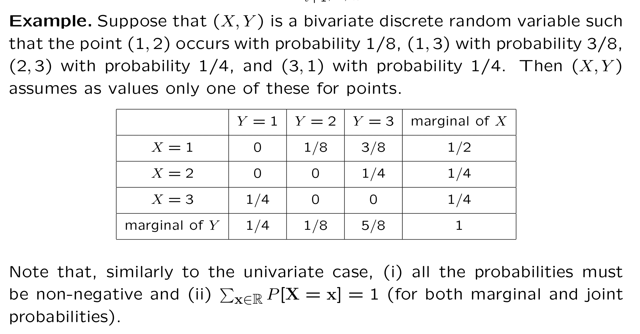
Definition 5.1 Let \(X\) and \(Y\) be a pair of discrete random variables
Their joint probability mass function (joint PMF) expresses the probability that simultaneously \(X\) takes on the specific value \(x\) and \(Y\) takes on the specific value \(y\).
It is denoted by \[\begin{equation*} p_{X,Y}\left( x,y\right) =\Pr (\left\{ X=x\cap Y=y\right\}) \end{equation*}\] thought of as a function of \(x\) and \(y\).The joint PMF has two essential properties:
The value of the Joint PMF is always non-negative \[p_{X,Y}\left( x,y\right) \geq 0 \text{ for all possible pairs }\left(x,y\right)\]
The sum over all combinations of \(x\) and \(y\) values is equal to one \[\sum_{x}\sum_{y}\Pr ( \left\{ X=x\cap Y=y\right\}) =1\]
Similarly, the probability (mass) function of the discrete random variable \(Y\) is called its marginal probability (mass) function. It is obtained by summing the joint probabilities relating to pairs \((X,Y)\) over all possible values of \(X\): \[\begin{equation*} p_{Y}(y)=\sum_{x}p_{X,Y}(x,y). \end{equation*}\]
Example 5.2 (caplets) Two caplets are selected at random from a bottle containing three aspirins, two sedatives and two placebo caplets. We are assuming that the caplets are well mixed and that each has an equal chance of being selected.
Let \(X\) and \(Y\) denote, respectively, the numbers of aspirin caplets, and the number of sedative caplets, included among the two caplets drawn from the bottle.
Number of sets of 2 caplets out of 7:
\[{7 \choose 2} = \frac{7!}{2!\times (7-2)!} = \frac{7!}{2! \times 5!} = \frac{6\times 7}{2} = 3\times 7 = 21\]
The Joint Probabilities can be found with Combinatorial Formulae:
- \(p_{X,Y}(0, 0) = {3 \choose 0}{2 \choose 0}{2 \choose 2} \left/ 21 \right. = 1/21\)
- \(p_{X,Y}(1, 0) = {3 \choose 1}{2 \choose 0}{2 \choose 1} \left/ 21 \right. = 6/21\)
- \(p_{X,Y}(2, 0) = {3 \choose 2}{2 \choose 0}{2 \choose 0} \left/ 21 \right. = 3/21\)
- \(p_{X,Y}(0, 1) = {3 \choose 0}{2 \choose 1}{2 \choose 1} \left/ 21 \right. = 4/21\)
- \(p_{X,Y}(1, 1) = {3 \choose 1}{2 \choose 1}{2 \choose 0} \left/ 21 \right. = 6/21\)
- \(p_{X,Y}(2, 1) = 0\) since \(2+1 = 3 > 2\)
- \(p_{X,Y}(0, 2) = {3 \choose 0}{2 \choose 2}{2 \choose 0} \left/ 21 \right. = 1/21\)
- \(p_{X,Y}(1, 2) = 0\) since \(1+2 = 3 > 2\)
- \(p_{X,Y}(2, 2) = 0\) since \(2+2 = 4 > 2\)
Notice that we can deduce the following Joint PMF: \[P(X=x \cap Y=y) = p(x, y) = \left\{ \begin{array}{ll} {3 \choose x}{2 \choose y}{2 \choose 2-x-y} \left/{7 \choose 2}\right. & x+y\leq 2\\ 0 &otherwise\end{array}\right.\]
Tabulating the joint probabilities as follows, we can easily work out the marginal probabilities
| \(x\) | \(0\) | \(1\) | \(2\) | \(\Pr \left\{ Y=y\right\}\) | |
|---|---|---|---|---|---|
| \(y\) | |||||
| \(0\) | \(1/21\) | \(6/21\) | \(3/21\) | \(10/21\) | |
| \(1\) | \(4/21\) | \(6/21\) | \(0\) | \(10/21\) | |
| \(2\) | \(1/21\) | \(0\) | \(0\) | \(1/21\) | |
| \(\Pr\left\{X=x\right\}\) | \(6/21\) | \(12/21\) | \(3/21\) | \(1\) |
Example 5.3 (Empirical Example) Two production lines manufacture a certain type of item. Suppose that the capacity (on any given day) is 5 items for Line I and 3 items for Line II.
Assume that the number of items actually produced by either production line varies from one day to the next.
Let \((X,Y)\) represent the 2-dimensional random variable yielding the number of items produced by and , respectively, on any one day.
In practical applications of this type the joint probability (mass) function \(\Pr(\{X=x\cap Y=y\})\) is unknown more often than not!
The joint probability (mass) function \(\Pr(\{X=x\cap Y=y\})\) for all possible values of \(x\) and \(y\) can be approximated however.
By the observing the long-run relative frequency with which different numbers of items are actually produced by either production line.
| \(x\) | \(0\) | \(1\) | \(2\) | \(3\) | \(4\) | \(5\) | \(\Pr \left\{ Y=y\right\}\) | |
|---|---|---|---|---|---|---|---|---|
| \(y\) | ||||||||
| \(0\) | \(0\) | \(0.01\) | \(0.03\) | \(0.05\) | \(0.07\) | \(0.09\) | \(0.25\) | |
| \(1\) | \(0.01\) | \(0.02\) | \(0.04\) | \(0.05\) | \(0.06\) | \(0.08\) | \(0.26\) | |
| \(2\) | \(0.01\) | \(0.03\) | \(0.05\) | \(0.05\) | \(0.05\) | \(0.06\) | \(0.25\) | |
| \(3\) | \(0.01\) | \(0.02\) | \(0.04\) | \(0.06\) | \(0.06\) | \(0.05\) | \(0.24\) | |
| ${ X=x} $ | \(0.03\) | \(0.08\) | \(0.16\) | \(0.21\) | \(0.24\) | \(0.28\) | \(1\) |
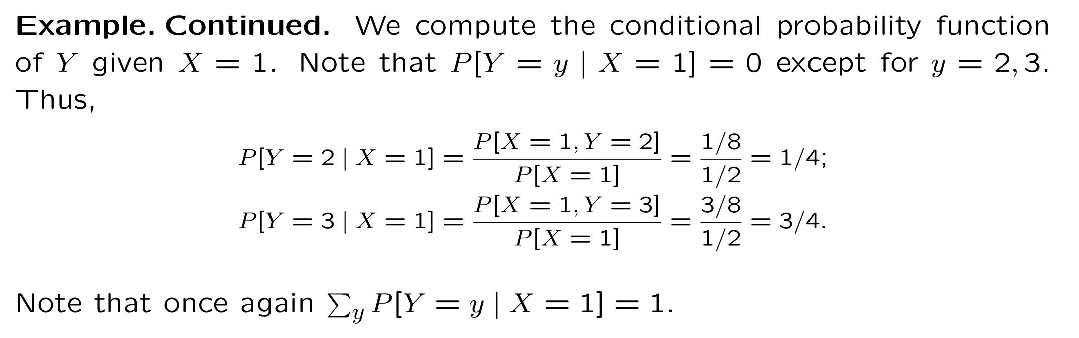
8.2 Conditional Probability
Recall that the conditional probability mass function of the discrete
random variable \(Y\), given that the random variable \(X\) takes the
value \(x\), is given by:
\[\begin{equation*}
p_{Y|X}\left( y|x\right) =\frac{\Pr \left\{ X=x\cap Y=y\right\} }{%
P_{X}\left( X=x\right) }
\end{equation*}\]
Note this is a probability mass function for \(y,\) with \(x\) viewed as fixed. Similarly:
Note this is a probability mass function for \(x,\) with \(y\) viewed as fixed.
8.2.1 Independence
Two discrete random variables \(X\) and \(Y\) are independent if \[\begin{eqnarray*} p_{X,Y}(x,y) &=&p_{X}(x)p_{Y}(y)\qquad \qquad \text{(discrete)} \\ %f_{X,Y}(x,y) &=&f_{X}(x)f_{Y}(y)\qquad \qquad \text{(continuous)} \end{eqnarray*}\] for values of \(x\) and \(y.\)
Note that independence also implies that \[\begin{eqnarray*} p_{X|Y}(x|y) &=&p_{X}(x)\text{ and }p_{Y|X}(y|x)=p_{Y}(y)\qquad \text{ (discrete)} \\ %f_{X|Y}(x|y) &=&f_{X}(x)\text{ and }f_{Y|X}(y|x)=f_{Y}(y)\qquad \text{ %(continuous)} \end{eqnarray*}\] for values of \(x\) and \(y\).
8.3 Expectations
Equivalently, the **conditional expectation }of \(h\left( X,Y\right)\) \(X=x\) is defined as: \[\begin{equation*} E\left[ h\left( X,Y\right) |x\right] =\sum_{y}h\left( x,y\right) p_{Y|X}\left( y|x\right). \end{equation*}\]
8.3.1 Iterated Expectations
This notation emphasises that whenever we write down \(E[\cdot]\) for an expectation we are taking that expectation with respect to the distribution implicit in the formulation of the argument.
The above formula is perhaps more easily understood using the more explicit notation: \[\begin{align*} E_{(X,Y)}[h(X,Y)]&=E_{(Y)}[E_{(X|Y)}[h(X,Y)]]\\ &=E_{(X)}[E_{(Y|X)}[h(X,Y)]] \end{align*}\]
This notation makes it clear what distribution is being used to evaluate the expectation, the joint, the marginal or the conditional.
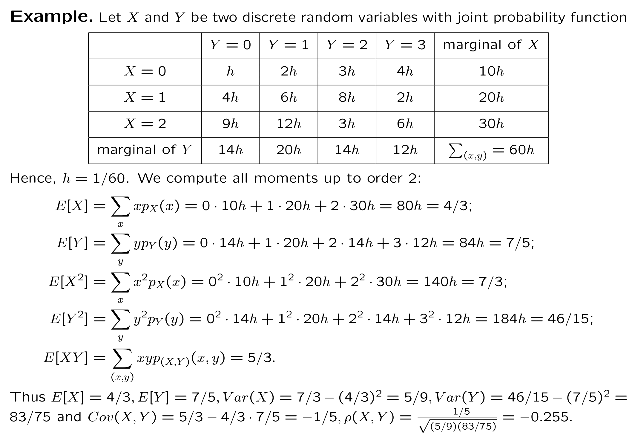
8.4 Covariance and Correlation
Alternative formula2 for \(Cov(X,Y)\) is \[\begin{equation} \boxed{Cov\left( X,Y\right) =E\left[ XY\right] -E\left[ X\right] E\left[ Y\right]\ .} \label{Cov} \end{equation}\]
So, to compute the covariance from a table describing the joint behaviour of \(X\) and \(Y\), you have to:
- compute the joint expectation \(E[XY]\)—you get it making use of the joint probability;
- compute \(E[X]\) and \(E[Y]\)—you get using the marginal probability for \(X\) and \(Y\);
- combine these expected values as in formula ().
See example on page 13 for an illustrative computation.
8.4.1 Some Properties of Covariances
The Cauchy-Schwartz Inequality states \[(E\left[ XY\right])^2\leq E\left[ X^2\right]E\left[ Y^2\right],\] with equality if, and only if, \(\Pr(Y=cX)=1\) for some constant \(c\).
Let \(h(a)=E[(Y-aX)^2]\) where \(a\) is any number. Then \[0\leq h(a)=E[(Y-aX)^2]=E[X^2]a^2-2E[XY]a+E[Y^2]\,.\]
This is a quadratic in \(a\), and
- if \(h(a)>0\) the roots are real and \(4(E[XY])^2-4E[X^2]E[Y^2]<0\),
- if \(h(a)=0\) for some \(a=c\) then \(E[(Y-cX)^2]=0\), which implies that \(\Pr(Y-cX=0)=1\).
Building on this remark, we have \(Cov(X,Y)>0\) if
large values of \(X\) tend to be associated with large values of \(Y\)
small values of \(X\) tend to be associated with small values of \(Y\)
\(Cov(X,Y)<0\) if
large values of \(X\) tend to be associated with values of \(Y\)
small values of \(X\) tend to be associated with values of \(Y\)
When \(Cov(X,Y)=0\), \(X\) and \(Y\) are said to be uncorrelated.
If \(X\) and \(Y\) are two random variables (either discrete or continuous) with \(Cov(X,Y) \neq 0\), then: \[\begin{equation} Var(X + Y) = Var(X) + Var(Y) + 2 Cov(X,Y) \label{FullVar} \end{equation}\]
, where we read that in the case of independent random variables \(X\) and \(Y\) we have \[Var(X + Y) = Var(X) + Var(Y),\] which trivially follows from ()—indeed, for independent random variables, \(Cov(X,Y)\equiv 0\).
- The covariance depends upon the unit of measurement.
8.4.2 A remark
- If we scale \(X\) and \(Y\), the covariance changes: For \(a,b>0\)% \[\begin{equation*} Cov\left( aX,bY\right) =abCov\left( X,Y\right) \end{equation*}\]
Thus, we introduce the correlation between \(X\) and \(Y\) is \[\begin{equation*} corr\left( X,Y\right) =\frac{Cov\left( X,Y\right) }{\sqrt{Var\left( X\right) Var\left( Y\right) }} \end{equation*}\]
which depend upon the unit of measurement.