5 🔧 Discrete Random Variables

Figure 3.1: ‘Alea Acta Est’ by Enrico Chavez

5.1 What is a Random Variable?

Up until now, we have considered probabilities associated with random experiments characterised by different types of events. For instance, we’ve illustrated events associated with experiments such as drawing a card (e.g. the card may be ‘hearts or diamonds’) or tossing a coin (e.g. the coins may show two heads ‘\(HH\)’). This has led us to characterise events as sets and, using set theory, compute the probability of combinations of sets, (e.g. an event in `\(A\cup B^{c}\)’).

To continue further in our path of formalising the theory of probability, we shall introduce the very important notion of Random Variable and start exploring Discrete Random Variables.

Definition 5.1 (Informal definition) Broadly speaking, a Random Variable is a variable that takes on different numerical values with various probabilities of occurrence associated with each different outcome.

Hence, to define a random variable, we need:

1. a list of all possible numerical outcomes, and
2. the probability for each numerical outcome

Example 5.1 (Rolling the dice - again) When we roll a single die, and record the number of dots on the top side, we can consider this the result of our draw as a Random Variable.

In this case, the list of all possible outcomes of this random process is the number shown on the die i.e. the possible outcomes are 1, 2, 3, 4, 5 and 6. If we say each outcome is equally likely, then the probability of each outcome must be 1/6

Example 5.2 (Flipping Coins - Again) If we flip a coin 10 times, and record the number of times T (tail) occurs, then the possible outcomes of the random process are:

\[\begin{equation*} \text{0, 1, 2, 3, 4, 5, 6, 7, 8, 9 and 10} \end{equation*}\]

We can associate a probability to each of these numbers and the probabilities are determined by the assumptions made about the coin flips, e.g.

• the value probability of a ‘tail’ appearing on a single coin flip
• whether this probability is the same for every coin flip
• whether the 10 coin flips are ‘independent’ of each other

Example 5.3 (Completing a test) Suppose we want to study the time taken by school students to complete a test. Let us assume that no student is given more than 2 hours to finish the test.

Here, we can define \(X=\) as the completion time (in minutes), and the possible values of the random variable \(X\) are contained in the interval

\[(0,120]=\{x:0<x\leq 120\}.\]

We then need to associate probabilities with all events we may wish to consider, such as \[P\left(\{ X\leq 15\}\right) \quad \text{or} \quad P\left(\{ X>60\}\right).\]

5.1.1 Formal definition of a random variable

Suppose we have:

1. A sample space \(\color{green}{S}\)

2. A probability measure (\(\color{green}{Pr}\)) defined “using the events” of \(\color{green}{S}\)

Let \(\color{blue}{X}(\color{green}{s})\) be a function that takes an element \(\color{green}{s}\in S\) and maps it to a number \(x\)

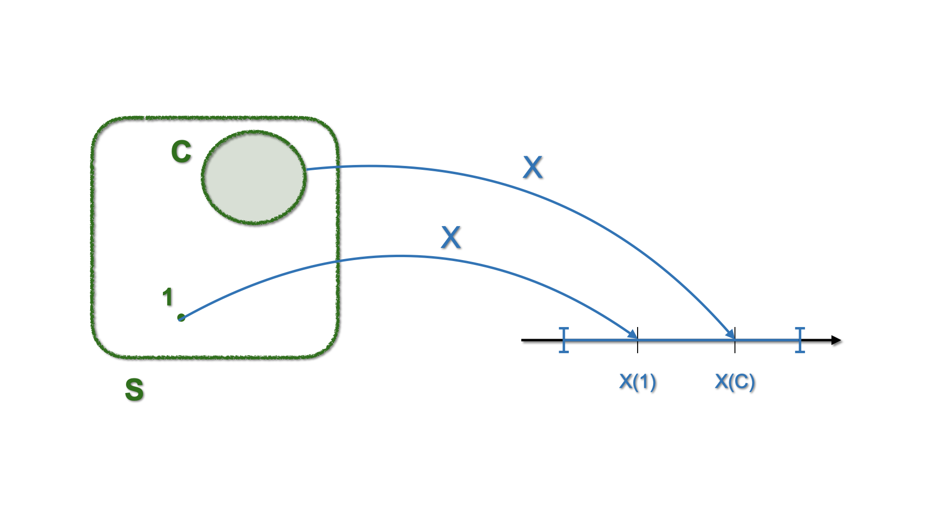
Figure 5.1: Schematic representation of mapping with a Random Variable

5.1.2 Example: from \(S\) to \(D\), via \(X(\cdot)\)

Example 1.1 (Rolling two dice) Consider the following Experiment: We roll two dice and we consider the number of points in the first die, and the number of points in the second die.

We already know that the sample space \({\color{green}S}\) is given by: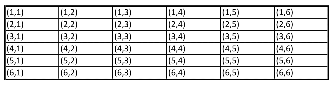

For the elements related to \(\color{green}S\) we have a probability \(\color{green}{Pr}\)

Now define \(X(\color{green}{s_{ij}})\) as the sum of the outcome \(i\) of the first die and the outcome \(j\) of the second die. Thus:

\[\begin{eqnarray*} X(\color{green}{s_{ij}})= X(i,j)= i+j, & \text{ for } & i=1,...,6, \text{ and } j=1,...,6 \end{eqnarray*}\]

In this notation \(\color{green}{s_{ij}=(i,j)}\) and \(\color{green}{s_{ij}\in S}\), each having probability \(1/36\).

Let us proceed to formalise this setting with a Random Variable and make the mapping explicit:

• \(X(\cdot)\) maps \(\color{green}{S}\) into \(\color{blue}D\). The (new) sample space \(\color{blue}{D}\) is given by: \[\begin{equation*} \color{blue}{D=\left\{2,3,4,5,6,7,8,9,10,11,12\right\}} \end{equation*}\] where, e.g., \(\color{blue}{2}\) is related to the pair \((1,1)\), \(\color{blue}{3}\) is related to the pairs \((1,2)\) and \((2,1)\), etc etc. So \(\color{blue}{D}\) is related the new \(\color{blue}{P}\)
• To each element (event) in \(\color{blue}{D}\) we can attach a probability, using the probability of the corresponding event(s) in \(S\). For instance, \[P(\color{blue}{2})=Pr(1,1)=1/36, \quad \text{or} \quad P(\color{blue}{3})=Pr(1,2)+Pr(2,1)=2/36.\]
• How about the \(P(\color{blue}{7})\)?
  \[\begin{equation*} P(\color{blue}7)=Pr(3,4)+Pr(2,5)+Pr(1,6)+Pr(4,3)+Pr(5,2)+Pr(6,1)=6/36. \end{equation*}\]
• The latter equality can also be re-written as \[P(\color{blue}7)=2(Pr(3,4)+Pr(2,5)+Pr(1,6))=6 \ Pr(3,4),\]

Exercise 1.1 1. What is \(P(\color{blue}{9})\)? 2. What is \(P(\color{blue} 13 )\)? [Hint: does \(\color{blue}{13}\) belong to \(\color{blue}{D}\)?]

Let us formalise all these ideas:

Definition 5.2 (A more formal definition) Let \(D\) be the set of all values \(x\) that can be obtained by \(X\left(s\right)\), for all \(s\in S\): \[\begin{equation*} D=\left\{ x:x=X\left( s\right) ,\text{ }s\in S\right\} \end{equation*}\] \(D\) is a list of all possible numbers \(x\) that can be obtained, and thus is a sample space for \(X\).

Notice that the random variable is \(X\) while \(x\) represents its realization i.e. “the value it takes”

\(D\) can be either:

• an uncountable interval, in which case,\(X\) is a continuous random variable, or
• a discrete or countable, in which case, \(X\) is a discrete random variable

For X to be a random variable it is required that for each event \(A\) consisting, if you will, of elements in \(D\): \[\begin{equation*} \color{blue}P\left( A\right) = \color{green} {Pr} ( \left\{ s\in S :X\left( s \right) \in A\right\}) \end{equation*}\] where \(\color{blue}{P}\) and \(\color{green}{Pr}\) stand for “probability” on \(\color{blue}{D}\) and on \(\color{green}{S}\), respectively, we assess the following properties (See Chapter 4):

• \(P \left( A\right) \geq 0\) %for all \(A\in \mathcal{B}_{D}\)
• \(\color{blue}P \left( D\right) =\color{green}Pr (\left\{ s\in S:X\left( s\right) \in D\right\}) =Pr \left( S\right) =1\)
• If \(A_{1},A_{2},A_{3}...\) is a sequence of events such that: \[A_{i}\cap A_{j}=\varnothing\] for all \(i\neq j\) then: \[\color{blue}P \left( \bigcup _{i=1}^{\infty }A_{i}\right) =\sum_{i=1}^{\infty } \color{blue} P\left( A_{i}\right).\]

In what follows we will be dropping the colors.

5.1.3 An Example from gambling

Example 4.2 (Geometric random variable) Let us imagine we are playing a game consisting of rolling a die until a 6 appears. Let us use \(X\) to denote the number of rolls required to obtain a 6. Hence, the possible values of \(X\) are: \(1, 2, 3,\ldots,n,\ldots\) (\(\equiv \mathbb{N}\)). Moreover, we can list the following probabilities associated with these values and the respective events:

• \(P(\{X=1\}) =\Pr (\text{obtain a 6 on the 1st roll})= \frac{1}{6}\)
• \(P (\{X=2\})=\Pr \left( \text{no }6\text{ on the 1st roll and }6\text{ on the 2nd roll}\right) =\frac{5}{6}\cdot \frac{1}{6}=\frac{5}{36}\)
• \(P(\{X=3\})=\Pr \left( \text{no }6\text{ on the 1st nor 2nd roll and '6' on the third roll}\right)\) \(=\frac{5}{6}\cdot \frac{5}{6}\cdot \frac{1}{6}=\frac{25}{216}\) and so on.

Here we start seeing a pattern or a recurrence and we can thus infer that the probability that it will take us \(n\) throws to obtain a 6 is given by:

\[\begin{align*} P(\{X=n\})&=\Pr(\text{no }6\text{ on the first } n-1 \text{ rolls and 6 on the last roll})\\ &=\left(\frac{5}{6}\right)^{n-1}\cdot \frac{1}{6} \end{align*}\]

This example also allows to see that rather than listing all the possible values of \(X\) along with the associated probabilities in a table, we can provide a formula that gives the required probabilities for a value \(X=n\). Hence, the probability function (a.k.a the Probability Mass Function (PMF)) of the random variable \(X\) is given by:

\[\begin{equation*} P(\left\{ X=n \right\})=\left(\frac{5}{6}\right)^{n-1}\frac{1}{6}\quad\text{for} \quad n=1,2,\ldots \end{equation*}\]

Finally, let’s also notice that this function fulfills the conditions to be a probability function. Using properties of geometric series, we can verify that:
\[\begin{equation*} \sum_{n=1}^\infty\left(\frac{5}{6}\right)^{n-1}\frac{1}{6}=1. \end{equation*}\]

5.2 Discrete random variables

Discrete random variables are often associated with the process of counting. The previous example is a good illustration of that use. More generally, we can characterise the probability of any random variable as follows:

Definition 5.3 (Probability of a Random Variable) Suppose \(X\) can take the values \(x_{1},x_{2},x_{3},\ldots ,x_{n}\). The probability of \(x_{i}\) is \[p_{i}= P(\left\{ X=x_i\right\})\]

and we must have \(p_{1}+p_{2}+p_{3}+\cdots +p_{n}=1\) and all \(p_{i}\geq 0\). These probabilities may be put in a table:

\(x_i\)	\(P(\left\{ X=x_i\right\})\)
\(x_{1}\)	\(p_{1}\)
\(x_{2}\)	\(p_{2}\)
\(x_{3}\)	\(p_{3}\)
\(\vdots\)	\(\vdots\)
\(x_{n}\)	\(p_{n}\)
Total	\(1\)

For a discrete random variable \(X\), any table listing all possible nonzero probabilities provides the entire probability distribution.

And the probability mass function \(p(a)\) of \(X\) is defined by: \[ p_a = p(a)= P(\{X=a \}), \] and this is positive for at most a countable number of values of \(a\). For instance, \(p_{1} = P(\left\{ X=x_1\right\})\), \(p_{2} = P(\left\{ X=x_2\right\})\), and so on.

That is, if \(X\) must assume one of the values \(x_1,x_2,...\), then \[\begin{eqnarray} p(x_i) \geq 0 & \text{for \ \ } i=1,2,... \\ p(x) = 0 & \text{otherwise.} \end{eqnarray}\]

Clearly, we must have \[ \sum_{i=1}^{\infty} p(x_i) = 1. \]

5.3 Cumulative Distribution Function

The cumulative distribution function (CDF) is a table listing the values that \(X\) can take, alongside the the cumulative probability, i.e. \[F_X(a) = P \left(\{ X\leq a\}\right)= \sum_{\text{all } x \leq a } p(x).\]

If the random variable \(X\) takes on values \(x_{1},x_{2},x_{3},\ldots .,x_{n}\) listed in increasing order \(x_{1}<x_{2}<x_{3}<\cdots <x_{n}\), the CDF is a step function, that it its value is constant in the intervals \((x_{i-1},x_i]\) and takes a step/jump of size \(p_i\) at each \(x_i\):

\(x_i\)	\(F_X(x_i)=P\left(\{ X\leq x_i\}\right)\)
\(x_{1}\)	\(p_{1}\)
\(x_{2}\)	\(p_{1}+p_{2}\)
\(x_{3}\)	\(p_{1}+p_{2}+p_{3}\)
\(\vdots\)	\(\vdots\)
\(x_{n}\)	\(p_{1}+p_{2}+\cdots +p_{n}=1\)

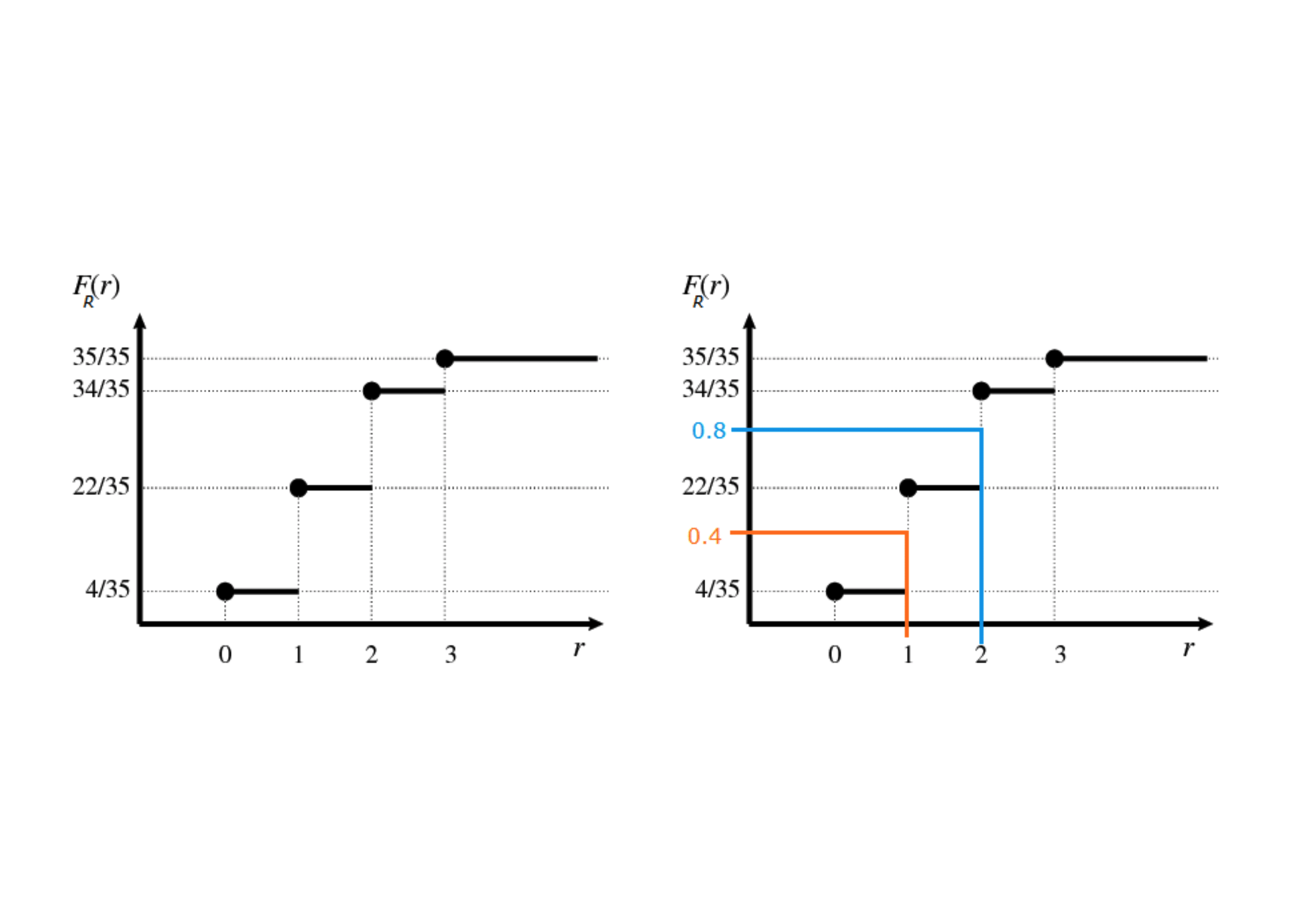
Example 5.4 Let us conside a random variable \(X_i\) taking values \(\{0,1,2,3\}\) with the probabilities listed as follows. We can display the values of the PDF and the PMF at the same time:

\(x_i\)	\(P(\{X=x_i\})\)	\(P(\{X\leq x_i\})\)
0	4/35	4/35
1	18/35	22/35
2	12/35	34/35
3	1/35	35/35
Total	1

Moreover, we can provide the expression of the CDF as a function defined on intervals: \[F_X(x) = \left\{ \begin{array}{ll} 0 & x<0 \\ 4/35 & 0 \leq x < 1\\ 22/35 & 1 \leq x < 2\\ 34/35 & 2 \leq x < 3 \\ 1 & x \geq 3. \end{array} \right.,\] which can be displayed graphically as a step function

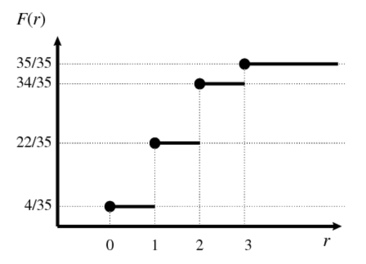
Figure 5.2: Step function

Remark. Suppose \(a\leq b\). Then, because the event \(\{X\leq a \}\) is contained in the event \(\{X\leq b \}\), namely \[\{X\leq a \} \subseteq \{X\leq b \},\] it follows that \[F_X(a) \leq F_X(b),\] so, the probability of the former is less than or equal to the probability of the latter. In other words, \(F_X(x)\) is a nondecreasing function of \(x\).

Example 5.5 (Quantiles) Since the CDF is monotonous, it can be inverted to define the value \(x\) of \(X\) that corresponds to a given probability \(\alpha\), namely \(\alpha = P (X \leq x )\), for \(\alpha \in [0,1]\).

The inverse CDF \(F_X^{-1}(\alpha)\) or quantile of order \(\alpha\), and labelled as \(Q(\alpha)\), is the smallest realisation of \(X\) associated to a CDF greater or equal to \(\alpha\); in formula, the \(\alpha\)-quantile \(Q(\alpha)\) is the smallest number satisfying: \[F_X [F^{-1}_X (\alpha)] = P[X \leq \underbrace{F^{-1}_X (\alpha)}_{Q(\alpha)}] \geq \alpha, \quad \text{for} \quad \alpha\in[0,1].\] By construction, a quantile of a discrete random variable is a realization of \(X\).

If we denote the random variable as \(R\), its realisations with \(r\) and the CDF evaluated in \(r\) as \(F_R(r)\), we can see graphically:

5.4 Distributional summaries for discrete random variables

In many applications, it is useful to describe some attributes or properties of the distribution of a Random Variable, for instance, to have an overview of how “central” a realisation is or how “spread” or variable the distribution really is. In this section, we will define two of these summaries:

• The Expectation, or Mean of the distribution is an indicator of “location.” It is defined as the mean of the realisations weighted by their probabilities, i.e.  \[\begin{equation*} E\left[ X\right] =p_{1}x_{1}+p_{2}x_{2}+\cdots + p_{n}x_{n} = \sum_{i=1}^{n} p_i x_i \end{equation*}\] Roughly speaking the mean represents the center of gravity of the distribution.

• The square root of the variance, or standard deviation, of the distribution is a measure of spread and is computed as the average squared distance between the observations with respect to the Expectation. \[\begin{eqnarray*} s.d\left( X\right) &=&\sqrt{Var\left( X\right) } \\ &=&\sqrt{p_{1}\left( x_{1}-E\left[ X\right] \right) ^{2}+p_{2}\left( x_{2}-E \left[ X\right] \right) ^{2}+\cdots + p_{n}\left( x_{n}-E\left[ X\right] \right) ^{2}} \end{eqnarray*}\] Roughly spread (or ‘variability’ or ‘dispersion’).

5.4.1 Properties

If \(X\) is a discrete random variable and \(a\) is any real number, then

• \(E\left[ \alpha X\right] =\alpha E\left[ X\right]\)
• \(E\left[ \alpha+X\right] =\alpha+E\left[ X\right]\)
• \(Var\left( \alpha X\right) =\alpha^{2}Var\left( X\right)\)
• \(Var\left( \alpha+X\right) =Var\left( X\right)\)

Exercise 3.7 Let us verify the first property: \(E\left[ \alpha X \right] =\alpha E\left[ X\right]\).

From the Intro lecture we know that, for every \(\alpha_i \in \mathbb{R}\),
\[\sum_{i=1}^{n} \alpha_i X_{i} = \alpha_1 X_1 + \alpha_2 X_2 +....+ \alpha_n X_n.\] So, the required result follows as a special case, setting \(\alpha_i= \alpha\), for every \(i\), and applying the definition of expected value.

Verify this and the other properties as an exercise. [Hint: set \(\alpha_i = \alpha p_i\).]

5.5 Dependence/Independence

Definition 5.4 Consider two discrete random variables \(X\) and \(Y\). Then, \(X\) and \(Y\) are independent if \[\begin{equation*} P \left(\left\{ \ X=x\right\} \cap \left\{ Y=y\right\} \right) =P \left(\{ X=x\}\right) \cdot P \left(\{ Y=y \}\right) \end{equation*}\] for all values \(x\) that \(X\) can take and all values \(y\) that \(Y\) can take.

5.5.1 More important properties

• If \(X\) and \(Y\) are two discrete random variables, then% \[\begin{equation*} E\left[ X+Y\right] =E\left[ X\right] +E\left[ Y\right] \end{equation*}\]

• If \(X\) and \(Y\) are also independent, then \[\begin{equation} Var\left( X+Y\right) =Var\left( X\right) +Var\left( Y\right) \label{Eq. Var} \end{equation}\]

Remark. Note that Eq. () does not (typically) hold if \(X\) and \(Y\) are NOT independent—more to come on this later on…

5.5.2 More on expectations

Recall that the expectation of X was defined as \[\begin{equation*} E\left[ X\right] = \sum_{i=1}^{n} p_i x_i \end{equation*}\]

Now, suppose we are interested in a function \(m\) of the random variable \(X\), say \(m(X)\). We define \[\begin{equation*} E\left[ m\left( X\right) \right] =p_{1}m\left( x_{1}\right) +p_{2}m\left( x_{2}\right) +\cdots p_{n}m\left( x_{n}\right). \end{equation*}\]

Notice that the variance is a special case of expectation where, \[\begin{equation*} m(X)=(X-E\left[ X\right] )^{2}. \end{equation*}\] Indeed, \[\begin{equation*} Var\left( X\right) =E\left[ (X-E\left[ X\right] )^{2}\right]. \end{equation*}\]

5.6 Some discrete distributions of interest

• Discrete Uniform
• Bernoulli
• Binomial
• Poisson
• Hypergeometric
• Negative binomial

Their main characteristic is that the probability \(P\left(\left\{ X=x_i\right\}\right)\) is given by an appropriate mathematical formula: i.e.  \[p_{i}=P\left(\left\{ X=x_i\right\}\right)=h(x_{i})\] for a suitably specified function \(h(\cdot)\).

5.6.1 Discrete uniform distribution

Definition 5.5 We say \(X\) has a discrete uniform distribution when

• \(X\) can take the values \(x=0,1,2,...,k\) (for some specified finite value \(k\in \mathbb{N}\))
• The probability that \(X=x\) is \(1/\left( k+1\right)\), namely

\[P\left(\left\{ X=x\right\}\right) = \frac{1}{\left( k+1\right)}.\]

The probability distribution is given by

\(x_i\)	\(P \left(\left\{ X=x_i\right\}\right)\)
\(0\)	\(\frac{1}{\left( k+1\right) }\)
\(1\)	\(\frac{1}{\left( k+1\right) }\)
\(\vdots\)	\(\vdots\)
\(k\)	\(\frac{1}{\left( k+1\right) }\)
Total	\(1\)

5.6.1.1 Expectation

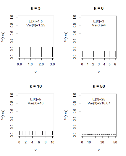
• The expected value of \(X\) is \[\begin{eqnarray*} E\left[ X\right] &=& x_1 p_1 + ... + x_k p_k\\ &=& 0\cdot \frac{1}{\left( k+1\right) }+1\cdot \frac{1}{% \left( k+1\right) }+\cdots +k\cdot \frac{1}{\left( k+1\right) } \\ &=&\frac{1}{\left( k+1\right) }\cdot\left( 0+1+\cdots +k\right) \\ &=&\frac{1}{\left( k+1\right) }\cdot \frac{k\left( k+1\right) }{2} \\ &=&\frac{k}{2}. \end{eqnarray*}\]

E.g. when \(k=6\), then \(X\) can take on one of the seven distinct values \(x=0,1,2,3,4,5,6,\) each with equal probability \(\frac{1}{7}\), but the expected value of \(X\) is equal to \(3\), which is one of the possible outcomes!!!

5.6.1.2 Variance

• The variance of \(X\) – we will be denoting it as \(Var(X)\) – is% \[\begin{eqnarray*} Var\left( X\right) &=&\left( 0-\frac{k}{2}\right) ^{2}\cdot \frac{1}{\left( k+1\right) }+\left( 1-\frac{k}{2}\right) ^{2}\cdot \frac{1}{\left( k+1\right) }+ \\ &&\cdots +\left( k-\frac{k}{2}\right) ^{2}\cdot \frac{1}{\left( k+1\right) } \\ &=&\frac{1}{\left( k+1\right) }\cdot\left\{ \left( 0-\frac{k}{2}\right) ^{2}+\left( 1-\frac{k}{2}\right) ^{2}+\cdots +\left( k-\frac{k}{2}\right) ^{2}\right\} \\ &=&\frac{1}{\left( k+1\right) }\cdot \frac{k\left( k+1\right) \left( k+2\right) }{12} \\ &=&\frac{k\left( k+2\right) }{12} \end{eqnarray*}\]

E.g. when \(k=6\), the variance of \(X\) is equal to \(4,\) and the standard deviation of \(X\) is equal to \(\sqrt{4}=2.\)

5.6.1.3 Illustrations

Example 4.5 An example of discrete uniform is related to the experiment of rolling a die- with the important remark that the outcome zero is not allowed in this specific example.

Let us call \(X\) the corresponding random variable and \(\{x_1,x_2,...,x_6\}\) its realizations.

The possible outcomes are: \[\{1,2,3,4,5,6\}\] each having probability \(\frac{1}{6}\).

Moreover, \[E(X) = (1+2+3+4+5+6) \cdot \frac{1}{6} = 3.5,\] which is not one of the possible outcomes(!)

5.6.2 Bernoulli Trials

Definition 5.6 Bernoulli trial is the name given to the random variable \(X\) having probability distribution given by

\(x_i\)	\(P(\left\{ X=x_i\right\})\)
\(1\)	\(p\)
\(0\)	\(1-p\)

Often we write the probability mass function (PMF) as:

\[\begin{equation*} P(\left\{ X=x\right\})=p^{x}\left( 1-p\right) ^{1-x}, \quad \text{ for }x=0,1 \end{equation*}\]

A Bernoulli trial represents the most primitive form of all random variables. It derives from a random experiment having only two possible mutually exclusive outcomes. These are often labelled Success and Failure and

• Success occurs with probability \(p\)
• Failure occurs with probability \(1-p\).

Remark. Just for the sake of notation, let us set \(X=1\) if Success occurs, and \(X=0\) if Failure occurs

Example 5.6 Coin tossing: we can define a random variable

\(x_i\)	\(P(\left\{ X=x_i\right\})\)
\(1\)	\(p\)
\(0\)	\(1-p\)

and say that \(X=1\) if \(H\) and \(X=0\) if \(T\).

5.6.2.1 Expectation

\[\begin{eqnarray*} E\left[ X\right] &=&1 \cdot p+0 \cdot (1-p) \\ &=&p \end{eqnarray*}\]

5.6.2.2 Variance

\[\begin{eqnarray*} Var\left( X\right) &=&\left( 1-p\right) ^{2} \cdot p+\left( 0-p\right) ^{2} \cdot \left( 1-p\right) \\ &=&p\left( 1-p\right). \end{eqnarray*}\]

5.6.3 The Binomial Distribution

Definition 5.7 Let us consider the random experiment consisting in a series of \(n\) trials having 3 characteristics

• Only two mutually exclusive outcomes are possible in each trial: success (S) and failure (F)
• The outcomes in the series of \(n\) trials constitute independent events
• The probability of success \(p\) in each trial is constant from trial to trial

\(X\) is the number of successes occurring in \(n\) (Bernoulli) trials. Binomial probability distribution given by: \[\begin{eqnarray} P(\left\{ X=x\right\})&=&{n \choose k} p^{x}\left(1-p\right)^{n-x} \\ &=&\frac{n!}{x!\left( n-x\right) !}p^{x}\left( 1-p\right) ^{n-x},\text{ for }% x=0,1,2,...,n \tag{5.1} \end{eqnarray}\]

You might recall from Chapter 1 that Combinations are defined as: \[\begin{equation*} {n \choose k} =\frac{n!}{k!\left( n-k\right) !}=C^{k}_{n} \end{equation*}\] and, for \(n \geq k\), we say ``\(n\) choose \(k\)’’.

The binomial coefficient \(n \choose k\) represents the number of possible combinations of \(n\) objects taken \(k\) at a time, without regard of the order. Thus, \(C^{k}_{n}\) represents the number of different groups of size \(k\) that could be selected from a set of \(n\) objects when the order of selection is not relevant.

So, “What is the interpretation of the formula?”

• The first factor \[{n \choose k} =\frac{n!}{x!\left( n-x\right)!}\] is the number of different combinations of individual “successes” and “failures” in \(n\) (Bernoulli) trials that result in a sequence containing a total of \(x\) ‘successes’ and \(n-x\) “failures.”
• The second factor \[p^{x}\left( 1-p\right) ^{n-x}\] is the probability associated with any one sequence of \(x\) ‘successes’ and \((n-x)\) `failures’.

Remark. Short-hand notation: \[X \sim \mathcal{B}(x,n,p)\] or, occasionally, simply $ X (n,p)$ (no \(x\) in the formula).

5.6.3.1 Expectation

\[\begin{eqnarray*} E\left[ X\right] &=&\sum_{x=0}^{n}x\Pr \left\{ X=x\right\} \\ &=&\sum_{x=0}^{n}x {n\choose k} p^{x}\left(1-p\right) ^{n-x} = np \end{eqnarray*}\]

5.6.3.2 Variance

\[\begin{eqnarray*} Var\left( X\right) &=&\sum_{x=0}^{n}\left( x-np\right) ^{2} P (\left\{ X=x\right\}) \\ &=&np\left( 1-p\right) \end{eqnarray*}\]

Remark. Looking at (@ref{eq:Binom}), we remark that the Bernoulli distribution is a special case (\(n=1\)) of the Binomial distribution. Roughly speaking, ``a Binomial random variable arises when we sum \(n\) independent Bernoulli trails.’’

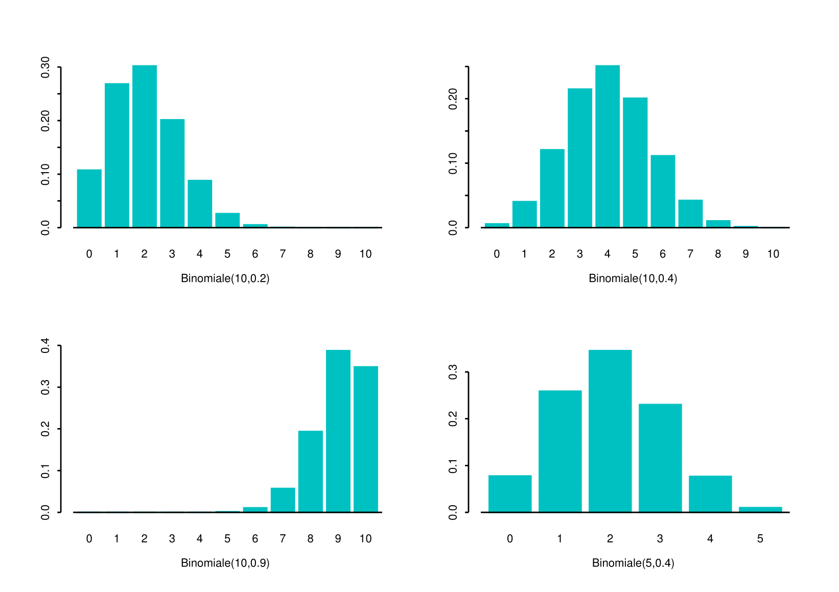
5.6.3.3 Illustrations

The visualisation shows some similiarities to the Discrete Uniform but some values seem more probable than others. Moreover, the shape of the distribution seems to vary according to the values of \(n\) and \(p\), i.e the parameters of the distribution.

Example 4.8 (cherry trees) One night a storm washes three cherries ashore on an island. For each cherry, there is a probability \(p=0.8\) that its seed will produce a tree. What is the probability that these three cherries will produce two trees?

First, we notice that this can be determined using a Bernoulli distribution. To this end, consider whether each seed will produce a tree as a sequence of \(n=3\) trials. For each cherry:

• either the cherry produces a tree (Success) or it does not (Failure);
• the event that a cherry produces a tree is independent from the event that any of the other two cherries produces a tree.
• The probability that a cherry produces a tree is the same for all three cherries

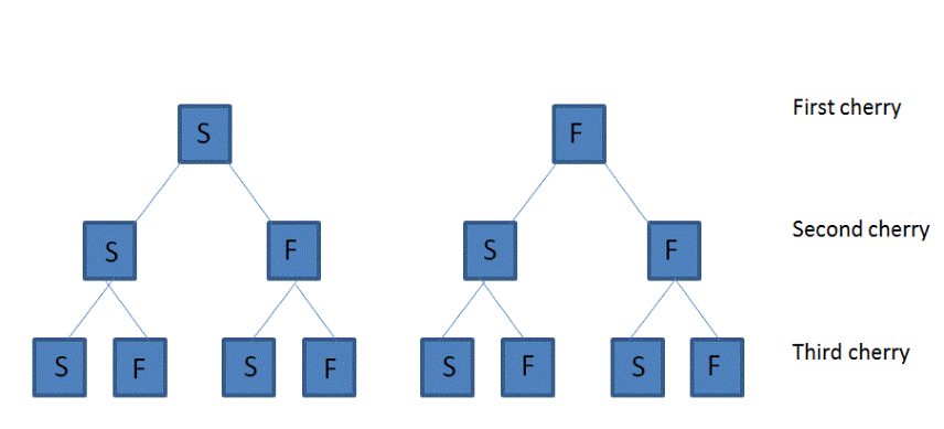
Example 5.7 - There are \(2^{3}=8\) possible outcomes from the \(3\) individual trials

• It does not matter which of the three cherries produce a tree

• Consider all of the possible sequences of outcomes (S=success, F=failure)

\[SSS, \color{red}{SSF}, \color{red}{SFS}, SFF, \color{red}{FSS, FSF, FFS, FFF}\]

• We are interested in \(\color{red}{SSF}\) , \(\color{red}{SFS}\), \(\color{red}{FSS}\)

• These possible events are mutually exclusive, so

\[\begin{equation*} \Pr(\left\{\color{red}{SSF} \cup \color{red}{SFS} \cup \color{red}{FSS} \right\}) = \Pr (\left\{\color{red}{SSF}\right\}) +\Pr (\left\{\color{red}{SFS}\right\}) + \Pr (\left\{\color{red}{FSS}\right\}) \end{equation*}\]

The three trials are assumed to be independent, so each of the three seed events corresponding to two trees growing has the same probability

\[\begin{eqnarray*} \Pr (\left\{\color{red}SSF \right\}) &=&\Pr (\left\{ \color{red}S \right\}) \cdot \Pr (\left\{\color{red} S\right\} ) \cdot (\Pr \left\{\color{red} F \right\} ) \\ &=&0.8\cdot 0.8\cdot (1-0.8) \\ &=&0.8\cdot (1-0.8)\cdot 0.8 =\Pr (\left\{\color{red}{SFS} \right\}) \\ &=&(1-0.8)\cdot 0.8\cdot 0.8= \Pr (\left\{\color{red}{FSS} \right\} ) \\ &=&0.128 \end{eqnarray*}\]

So the probability of two trees resulting from the three seeds must be

\[\begin{eqnarray*} \Pr (\left\{ \color{red}{SSF} \cup \color{red}{SFS} \cup \color{red}{FSS} \right\} ) &=&3\cdot 0.128 \\ &=&0.384. \end{eqnarray*}\]

Example 5.8 Finally, we notice that we can obtain the same result (in a more direct way), using the binomial probability for the random variable \[X= \text{number of trees that grows from 3 seeds}.\]

Indeed

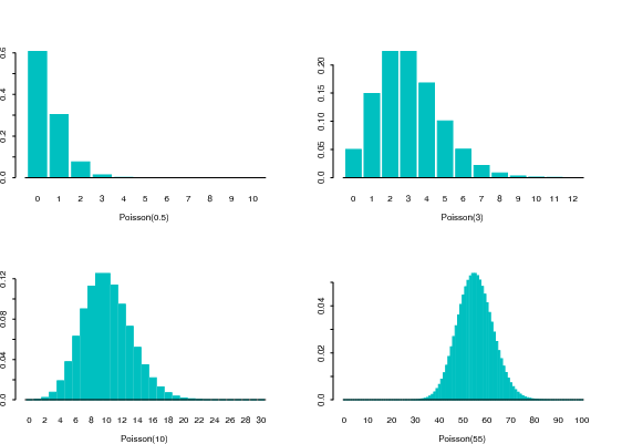
\[\begin{eqnarray*} \Pr (\left\{ X=2\right\}) &=&\frac{3!}{2!\left( 3-2\right) !}\cdot \left( 0.8\right) ^{2} \cdot \left( 1-0.8\right) ^{3-2} \\ &=&3 \cdot \left( 0.8\right) ^{2} \cdot \left( 0.2\right) \\ &=&0.384. \end{eqnarray*}\]

5.6.4 Poisson Distribution

Definition 5.8 Let us consider random variable \(X\) which takes values \(0,1,2,...\), namely the nonnegative integers in \(\mathbb{N}\). \(X\) is said to be a Poisson random variable if its probability mass function, with \(\lambda >0\) fixed and providing info on the intensity, is \[\begin{equation} p(x)=\Pr \left( \{ X = x \}\right) =\frac{\lambda ^{x}e^{-\lambda }}{x!}\text{,\qquad }% x=0,1,2,... \label{Eq. Poisson} \end{equation}\] and we write \(X\sim \text{Poisson}(\lambda)\).

The Eq. () defines a genuine probability mass function, since \(p(x) \geq 0\) and

\[\begin{eqnarray} \sum_{x=0}^{\infty} p(x) &=& \sum_{x=0}^{\infty} \frac{\lambda ^{x}e^{-\lambda }}{x!} \\ & = & e^{-\lambda } \sum_{x=0}^{\infty} \frac{\lambda ^{x}}{x!} \\ & = & e^{-\lambda } e^{\lambda } = 1 \quad \text{(see Intro Lecture).} \end{eqnarray}\]

Moreover, for a given value of $$ also the CDF can be easily defined. E.g.

\[\begin{equation*} F_X(2)=\Pr \left( \{X\leq 2\}\right) =e^{-\lambda }+\lambda e^{-\lambda }+\frac{\lambda ^{2}e^{-\lambda }}{2}, \end{equation*}\]

and the Expected value and Variance for Poisson distribution (see tutorial) can be obtained by ‘’sum algebra’’ (and/or some algebra)

\[\begin{eqnarray*} E\left[ X\right] &=&\lambda \\ Var\left( X\right) &=&\lambda. \end{eqnarray*}\]

5.6.4.1 Illustrations

… same barplot as in slide 30, just a bit fancier…

Example 5.9 The average number of newspapers sold by Alfred is 5 per minute. What is the probability that Alfred will sell at least 1 newspaper in a minute?

To answer, let \(X\) be the \(\#\) of newspapers sold by Alfred in a minute. We have

\[ X \sim \text{Poisson}(\lambda) \]

with \(\lambda = 5\), so \[\begin{eqnarray*} P(X \geq 1) & = & 1- P(\{X=0\}) \\ & = & 1 - \exp^{-5} \frac{5^0}{0!} \\ %& = & 1-\exp^{-5} \\ & \approx & 1- 0.0067 \approx 99.33\%. \end{eqnarray*}\] How about \(P(X \geq 2)\)? Is it \(P(X \geq 2) \geq P(X \geq 1)\) or not? Answer the question…

Example 5.10 A telephone switchboard handles 300 calls, on the average, during one hour. The board can make maximum 10 connections per minute. Use the Poisson distribution to evaluate the probability that the board will be overtaxed during a given minute.

To answer, let us set \(\lambda = 300\) per hour, which is equivalent to 5 calls per minute. Noe let us define \[ X = \text{\# of connections in a minute} \] and by assumption we have \(X \sim \text{Poisson}(\lambda)\). Thus, \[\begin{eqnarray} P[\text{overtaxed}] &=& P(\{X > 10\}) \\ &=& 1 \quad - \underbrace{P(\{X \leq 10\})}_{\text{using $\lambda=5$, minute base}} \\ &\approx& 0.0137. \end{eqnarray}\]

5.6.4.2 Link to Binomial

Let us consider \(X \sim B(x,n,p)\), where \(n\) is large, \(p\) is small, and the product \(np\) is appreciable. Setting, \(\lambda=np\), we then have that, for the Binomial probability as in Eq.(), it is a good approximation to write: \[ p(k) = P(\{X=k\}) \approx \frac{\lambda^k}{k!} e^{-\lambda}. \] To see this, remember that
\[ \lim_{n\rightarrow\infty} \left( 1- \frac{\lambda}{n} \right)^n = e^{-\lambda}. \] Then, let us consider that in our setting, we have \(p=\lambda/n\). From the formula of the binomial probability mass function we have: \[ p(0) = (1-p)^{n}=\left( 1- \frac{\lambda}{n} \right)^{n} \approx e^{-\lambda}, \quad \text{\ as \ \ } n\rightarrow\infty. \]

Moreover, it is easily found that

\[\begin{eqnarray} \frac{p(k)}{p(k-1)} &=& \frac{np-(k-1)p}{k(1-p)} \approx \frac{\lambda}{k}, \quad \text{\ as \ \ } n\rightarrow\infty. \end{eqnarray}\]

Therefore, we have

\[\begin{eqnarray} p(1) &\approx& \frac{\lambda}{1!}p(0) \approx \lambda e^{-\lambda} \\ p(2) &\approx& \frac{\lambda}{2!}p(1) \approx \frac{\lambda^2}{2} e^{-\lambda} \\ \dotsm & \dotsm & \dotsm \\ p(k) &\approx& \frac{\lambda}{k!}p(k-1) \approx \underbrace{\frac{\lambda^k}{k!} e^{-\lambda}}_{\text{\ see \ \ Eq. (\ref{Eq. Poisson}) }} \end{eqnarray}\]

thus, we remark that \(p(k)\) can be approximated by the probability mass function of a Poisson—which is easier to implement.

Example 5.11 (two-fold use of Poisson) Suppose a certain high-speed printer makes errors at random on printed paper. Assuming that the Poisson distribution with parameter \(\lambda = 4\) is appropriate to model the number of errors per page (say, \(X\)), what is the probability that in a book containing 300 pages (produced by the printer) at least 7 will have no errors?

Let \(X\) denote the number of errors per page, so that \[ p(x) = \exp^{-4}\frac{4^x}{x!}, \quad \text{for} \quad x = 0,1,2,.... \] The probability of any page to be error free is then \[p(0) = \exp^{-4}\frac{4^0}{0!} = \exp^{-4} \approx 0.018.\]

Having no errors on a page is a success, and there are 300 independent pages. Hence, let us define

\[ Y = \text{the number of pages without any errors}. \]

\(Y\) is binomially distributed with parameters \(n = 300\) and \(p = 0.018\), namely \[Y\sim B(n,p).\]

But here we have

thus, we can compute \(P(\{Y \geq 7\})\) using either the exact Binomial or its Poisson approximation. So

• using \(B(300,0.018)\), we get: \(P(\{Y \geq 7\}) \approx 0.297\)

• using Poisson(5.4), we get \(P(\{Y \geq 7\}) \approx 0.298.\)

5.6.5 The Hypergeometric Distribution

Definition 5.9 Let us consider a random experiment consisting of a series of \(n\) trials, having the following properties

• Only two mutually exclusive outcomes are possible in each trials: success (S) and failure (F)

• The population has \(N\) elements in which \(k\) are looked upon as S and the other \(N-k\) are looked upon as F

• Sampling from the population is done without replacement (so that the trials are not independent).

The random variable \[X= \text{number of successes in $n$ such trials}\] has an hypergeometric distribution and the probability that \(X=x\) is

\[\begin{equation*} \Pr (\left\{ X=x\right\}) =\frac{\left( \begin{array}{c} k \\ x% \end{array} \right) \left( \begin{array}{c} N-k \\ n-x \end{array} \right) }{\left( \begin{array}{c} N \\ n \end{array} \right)}. \end{equation*}\]

Moreover,

\[\begin{eqnarray*} E\left[ X\right] &=&\frac{nk}{N} \\ Var\left( X\right) &=&\frac{nk\left( N-k\right) \left( N-n\right) }{% N^{2}\left( N-1\right) } \end{eqnarray*}\]

5.6.5.1 Illustrations

Example 5.12 [Psychological experiment]

A group of 8 students includes 5 women and 3 men: 3 students are randomly chosen to participate in a psychological experiment. What is the probability that exactly 2 women will be included in the sample?%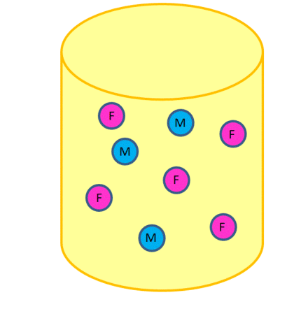

Consider each of the three participants being selected as a separate trial $$ there are \(n=3\) trials. Consider a woman being selected in a trial as a `success’ \ Then here \(N=8\), \(k=5\), \(n=3\), and \(x=2\), so that% \[\begin{eqnarray*} \Pr (\left\{ X=2\right\}) &=&\frac{\left( \begin{array}{c} 5 \\ 2% \end{array}% \right) \left( \begin{array}{c} 8-5 \\ 3-2% \end{array}% \right) }{\left( \begin{array}{c} 8 \\ 3% \end{array}% \right) } \\ && \\ &=&\frac{\frac{5!}{2!3!}\frac{3!}{1!2!}}{\frac{8!}{5!3!}} \\ && \\ &=&0.53571 \end{eqnarray*}\]

5.6.6 The Negative Binomial Distribution

Let us consider a random experiment consisting of a series of trials, having the following properties

• Only two mutually exclusive outcomes are possible in each trial: success' (S) andfailure’ (F)

• The outcomes in the series of trials constitute independent events

• The probability of success \(p\) in each trial is constant from trial to trial

What is the probability of having exactly \(y\) F’s before the \(r^{th}\) S?

Equivalently: What is the probability that in a sequence of \(y+r\) (Bernoulli) trials the last trial yields the \(r^{th}\) S?

Definition 5.10 Let \[X= \text{the total number of trials required until a total of $r$ successes is accumulated}.\] Then \(X\) is said to be a Negative Binomial random variable and its probability mass function
\(\Pr (\left\{ X=n\right\})\) equals the probability of \(r-1\) ‘successes’ in the first \(n-1\) trials, times the probability of a ‘success’ on the last trial. These probabilities are given by% \[\begin{equation*} \Pr (\left\{ X=n\right\}) =\left( \begin{array}{c} n-1 \\ r-1 \end{array} \right) p^{r}\left( 1-p\right) ^{n-r}\quad \text{ for }n=r,r+1,... \end{equation*}\]

The mean and variance for \(X\) are, respectively,%

\[\begin{eqnarray*} E\left[ X\right] &=&\frac{r}{p} \\ Var\left( X\right) &=&\frac{r\left( 1-p\right) }{p^{2}} \end{eqnarray*}\]

5.6.7 Illustrations

Example 5.13 [marketing research]

• A marketing researcher wants to find 5 people to join her focus group

• Let \(p\) denote the probability that a randomly selected individual agrees to participate in the focus group

• If \(p=0.2\), what is the probability that the researcher must ask 15 individuals before 5 are found who agree to participate?

%- That is, what is the probability that 10 people will decline the %request to participate before a 5\(^{th}\) person agrees?

• In this case, \(p=0.2\), \(r=5\), \(n=15\): we are looking for \(\Pr (\left\{ X=15\right\}).\) By the negative binomial formula we have

\[\begin{eqnarray*} \Pr (\left\{ X=15\right\}) &=&\left( \begin{array}{c} 14 \\ 4% \end{array}% \right) \left( 0.2\right) ^{5}\left( 0.8\right) ^{10} \\ &=&0.034 \end{eqnarray*}\]

5.6.8 The Geometric Distribution

Definition 5.11 (a special case) When \(r=1\), the negative binomial distribution is equivalent to the Geometric distribution

In this case, probabilities are given by \[\begin{equation*} \Pr (\left\{ X=n\right\}) =p\left( 1-p\right) ^{n-1}\text{, for }n=1,2,... \end{equation*}\]

The corresponding mean and variance for \(X\) are, respectively,

\[\begin{eqnarray*} E\left[ X\right] &=&\frac{ 1 }{p} \\ Var\left( X\right) &=&\frac{\left( 1-p\right) }{p^{2}} \end{eqnarray*}\]

Example 5.14 (failure of a machine) Items are produced by a machine having a 3% defective rate.

• What is the probability that the first defective occurs in the fifth item inspected? \[\begin{eqnarray} P(\{X = 5\}) &=& P (\text{first 4 non-defective}) P (\text{5th defective}) &=& (0.97)^4(0.03) \approx 0.026 \end{eqnarray}\]
• What is the probability that the first defective occurs in the first five inspections? \[\begin{eqnarray} P(\{X \leq 5 \}) = P(\{X < 6 \}) &=& P (\{X=1\})+ ... + P(\{X=5\}) &=& 1- P(\text{first 5 non-defective}) = 0.1412. %&=& 1- (0.97)^5 \approx 0.1412 \end{eqnarray}\]

More generally, for a geometric random variable we have:

\[P(\{X \geq k \}) = (1-p)^{k-1}\]

Thus, in the example we have \(P( \{X \geq 6 \}) = (1-0.03)^{6-1}\approx 0.8587\)

\[\begin{eqnarray} P(\{X \leq 5\}) = 1-P( \{X \geq 6 \}) \approx 1- 0.8587 \approx 0.1412. \end{eqnarray}\]